Offset Function in Excel revolutionizes data manipulation by dynamically referencing ranges based on specified parameters. This powerful function allows users to fetch data from adjacent cells, creating dynamic formulas that automatically adjust as the spreadsheet evolves. With the Offset Function in Excel, users can navigate through data sets, extract subsets, and perform complex calculations with precision and ease. Whether it’s building dynamic charts, automating reports, or conducting what-if analyses, mastering the Offset Function empowers users to unlock the full potential of their data. Stay ahead in your Excel game by harnessing the transformative capabilities of the Offset Function in Excel.
This Tutorial Covers:
- Define the OFFSET function in Excel
- Syntax of OFFSET function in Excel
- Arguments of OFFSET function in Excel
- Remarks
- Why should the OFFSET function be used and when should it be used in Excel
- How to use the OFFSET Function in Excel
- -Example 1–End Point is a Data Cell
- -Example 2–End Point is an Empty Cell
- -Example 3–End Point is a Non-existent Cell
- -Example 4–Sum of Values of the Returned Range Address
- -Example 5–Average of Values of the Returned Range Address
- Range Returned by the OFFSET Excel Function
1. Define the OFFSET function in Excel:
The value of a cell or range (of adjacent cells) that is a specific number of rows and columns from the reference point is returned by the OFFSET function in Excel. The initial cell given to the function as a parameter serves as this reference point. The function calculates an end point (finishing cell or range) starting from the reference point and returns its value.
-
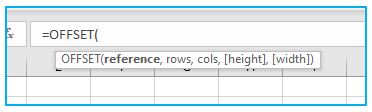
Syntax of OFFSET function in Excel: reference, rows, cols, height, and width
The following is the syntax for the OFFSET function in Microsoft Excel:
=OFFSET(reference, rows, cols, [height], [width])
-
Arguments of OFFSET function in Excel:
The OFFSET function in Microsoft Excel takes the following arguments:
reference: This is the starting point or cell from which you want to offset. It can be a cell reference or a named range (single cell or a range).
rows: This is the number of rows you want to offset. It can be a positive or negative number. For example, if you want to offset the reference cell by 3 rows down, you will use the value 3. If you want to offset it by 3 rows up, you will use the value -3.
columns: This is the number of columns you want to offset. It can also be a positive or negative number. For example, if you want to offset the reference cell by 2 columns to the right, you will use the value 2. If you want to offset it by 2 columns to the left, you will use the value -2.
height (optional): This is the number of rows you want to include in the range. It defaults to 1 if not specified.
width (optional): This is the number of columns you want to include in the range. It also defaults to 1 if not specified.
2. Remarks:
- OFFSET returns the #REF! error value if rows and cols offset reference goes beyond the margin of the worksheet.
- Height and width are presumed to be the same as reference if they are omitted.
- OFFSET only returns a reference; it doesn’t really move any cells or alter the selection. Any function that expects a reference argument can use OFFSET. One row beneath and two columns to the right of cell C2 is a 3-row by 1-column range, and the formula SUM(OFFSET(C2,1,2,3,1)) determines the total value of this range.
3. Why and when should the Excel OFFSET function be used?
The OFFSET formula in Excel is a powerful tool that allows users to reference a range of cells based on a specified number of rows and columns away from a starting point. It is particularly useful when working with large data sets or when dealing with dynamic data where the size or location of the data changes frequently.
The Excel OFFSET function can be used in a variety of scenarios, such as:
- Dynamic named range references: You can use the OFFSET function to create a dynamic range reference that expands or contracts automatically as the data changes.
- Conditional formatting: You can use the OFFSET function to reference a range of cells that need to be formatted based on certain conditions or criteria.
- Chart data series: You can use the OFFSET function to define a data series for a chart that automatically updates as new data is added or removed.
- Calculations: You can use the OFFSET function in complex calculations that require referencing specific cells or ranges of cells.
Overall, the OFFSET function is a versatile tool that can be used in many different scenarios to improve the efficiency and accuracy of your Excel work. It is particularly useful when dealing with dynamic data or when you need to create flexible range references.
Also Read: How to use INDEX and MATCH functions in Excel?
4. How to use OFFSET Function in Excel?
Excel comes with a built-in function called OFFSET. To use offset in Excel, let’s examine its operation with the aid of a few illustrations.
Each example includes an explanation of the OFFSET excel function and covers a distinct use scenario. The OFFSET function has been integrated with the arithmetic functions in the final two examples (examples 4 and 5).
-
Example 1–End Point is a Data Cell:
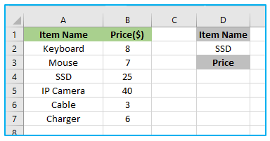
In this example, we have a table of six items and their prices, and we want to use the Excel OFFSET formula to find the price of the item named SSD.
The steps to use OFFSET function in Excel to find value where end point is a data cell are described below:
Step 1: Apply the following OFFSET formula in cell D4.
=OFFSET(A2,2,1)
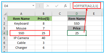
The result can be seen in cell D4. Therefore, “25” represents the price of the SSD item. The offset function in Excel returns the price of the item SSS.
Explanation:
Cell A2 serves as the reference point (beginning point) and is the initial argument to the OFFSET excel function.
The “rows” argument is 2. So, the function moves two rows below cell A2, which is the cell A4. The “cols” argument is 1. So, the function moves one column to the right of cell A2, which is the cell B4.
The value of the resulting cell (end point) B4 is “25.” Hence, the output in cell D4 is “25.” The end point is shown in the above image.
-
Example 2–End Point is an Empty Cell:
We want the OFFSET function to return the value of the blank cell C4 using the same dataset.
The steps to use OFFSET function in Excel to find value where end point is an empty cell are described below:
Step 1: Apply the below formula in cell D2.
=OFFSET(A2,2,2)
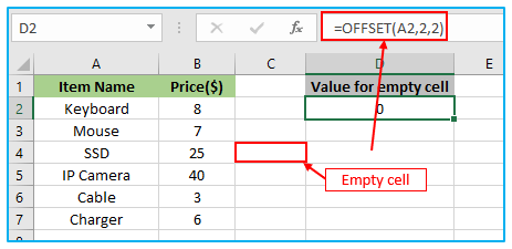
The result 0 is displayed in cell D2. As a result, the OFFSET method returns 0 for an empty cell’s value.
Explanation:
The reference point (beginning point) in the provided OFFSET excel formula is cell A2.
Since the “rows” argument is set to 2, cell A4 is moved down two rows by the function. The “cols” argument is also 2. So, the function moves two columns to the right of cell A2, which is the cell C4.
The resulting cell (end point) is C4. The OFFSET function’s output was set to 0 because this cell is empty. The end point is shown in the above
-
Example 3–End Point is a Non-existent Cell:
We want the OFFSET function to return the value of a nonexistent cell (directly to the left of cell A1) using the same dataset.
The steps to use OFFSET function in Excel to find value where end point is a non-existent cell are described below:
Step 1: Enter the following OFFSET excel formula in cell D2.
=OFFSET(A2,-1,-1)
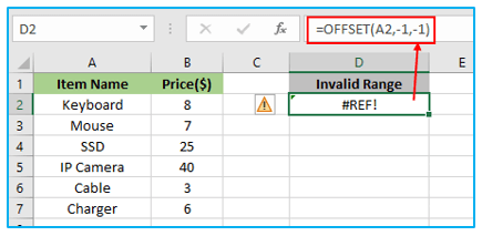
The result is displayed in cell D2. Therefore, the value of a missing cell is a “#REF!” error.
Explanation:
The reference point in this illustration is cell A2.
The argument for “rows” is -1. The function then advances one row above cell A2, which is cell A1, to the new location. Also -1 is the “cols” argument. As a result, cell A2 is moved one column to the left by the function. There isn’t a column to the left of column A, though.
As a result, there is no cell (end point) produced. The result is an error that says “#REF!” as seen in the following image. The yellow icon reads “invalid cell reference error.”
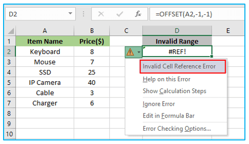
Note: A “#REF” error is returned by the OFFSET function if the end point belongs to a cell that is invalid or nonexistent.
-
Example 4–Sum of Values of the Returned Range Address: height and width arguments
Suppose you have a dataset that contains the monthly sales data for a business, as shown below:
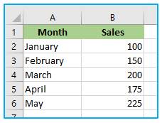
We can use the OFFSET function to create a formula that calculates the total sales for the first three months of the year (i.e., January, February, and March).
The steps to use OFFSET function in Excel to sum of values of the returned range address are described below:
Step 1: We can select an empty cell, such as cell D2, and enter the following formula:
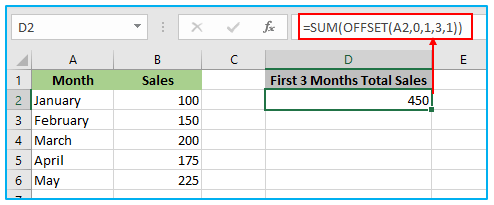
=SUM(OFFSET(A2,0,1,3,1))
Explanation:
This formula starts at cell A2 (the reference cell), offsets 0 rows and 1 column to the right (to skip the Month column) and returns a range that includes 3 rows (for January, February, and March) and 1 column (for the Sales data).
The SUM function then adds up the values in this range to give us the total sales for the first three months of the year, which is 450.
As new data is added to the table, the OFFSET function will automatically adjust to include the correct data for the first three months of the year. This makes the formula flexible and dynamic, which can save time and effort in updating formulas manually. Height and width arguments are used.
-
Example 5–Average of Values of the Returned Range Address:
Using the same dataset from example 4, we want to determine the average sales for the first three months. Use the AVERAGE function along with the OFFSET Excel function.
The steps to use OFFSET function in Excel to average of values of the returned range address are described below:
Step 1: Apply the following formula in cell D4.
=AVERAGE(OFFSET(A2,0,1,3,1))
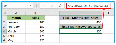
The result can be seen in cell D4. Thus, 150 sales were made on average during the first three months.
Explanation:
The first argument of the OFFSET function is A2, which is the reference cell, and is the starting point of the formula.
The second argument of the OFFSET function is 0, which means that we don’t want to move up or down from the reference cell.
The third argument of the OFFSET function is 1, which means that we want to move one column to the right of the reference cell (i.e., to cell B2).
The fourth argument of the OFFSET function is 3, which means that we want to include a range of three rows below the reference cell (i.e., cells B2, B3, and B4).
The fifth argument of the OFFSET function is 1, which means that we want to include a range of one column (i.e., only column B).
The OFFSET function returns a range of cells that includes B2, B3, and B4.
The AVERAGE function then calculates the average of the values in this range, which is (100+150+200)/3 = 150.
Therefore, the formula =AVERAGE(OFFSET(A2,0,1,3,1)) returns the value of 150, which is the average of the values in the range B2:B4.
Also Read: How to use Intersect Operator in Excel?
5. Range Returned by the OFFSET Excel Function:
To return the values of a range of adjacent cells using the OFFSET function in Excel, follow these steps:
- Select a blank range of cells that is the same size as the range you want to return.
- Enter the OFFSET formula in the upper-left cell of the blank range.
- Instead of just pressing Enter, press “Ctrl+Shift+Enter” to enter the formula as an array formula. This will cause curly brackets to appear at the beginning and end of the formula.
The values of the range of cells will be obtained as the output of the OFFSET function.
Note that to obtain the values of a range of cells, you must supply the “height” (number of rows) and “width” (number of columns) arguments in the OFFSET function.
Application of Offset Function in Excel
- Dynamic Range Selection: Use the OFFSET function to dynamically select a range of cells based on specified parameters, enabling flexible data analysis and reporting.
- Scrolling Data Display: Implement the OFFSET function to create scrolling data displays, where a user-defined range shifts based on scroll position, facilitating interactive dashboards.
- Dynamic Charting: Utilize OFFSET to dynamically adjust chart data ranges as new data is added, ensuring charts automatically update without manual intervention.
- Conditional Formatting: Apply OFFSET within conditional formatting rules to dynamically format cells based on changing criteria, enhancing data visualization and analysis.
- Dynamic Summaries: Employ OFFSET to generate dynamic summaries and totals from variable data ranges, enabling real-time insights into changing datasets.
- Interactive Dashboards: Create interactive dashboards by using OFFSET to display different sections of data based on user-selected criteria, enhancing data exploration capabilities.
For ready-to-use Dashboard Templates:
