Conditional Formatting in Excel is a powerful tool that allows users to visually highlight important trends, patterns, and outliers in their data. By applying formatting rules based on specified conditions, such as value ranges or specific criteria, users can quickly identify and analyze key insights within their spreadsheets. Whether it’s highlighting cells with the highest or lowest values, identifying duplicates, or flagging data that meets certain criteria, Conditional Formatting empowers users to make informed decisions and effectively communicate their findings. With its versatility and ease of use, Conditional Formatting in Excel is an essential feature for anyone looking to gain deeper insights from their data.
How to use Excel’s conditional formatting?
There are several ways you can apply conditional formatting in your worksheet.
Conditional Formatting from the HOME menu tab
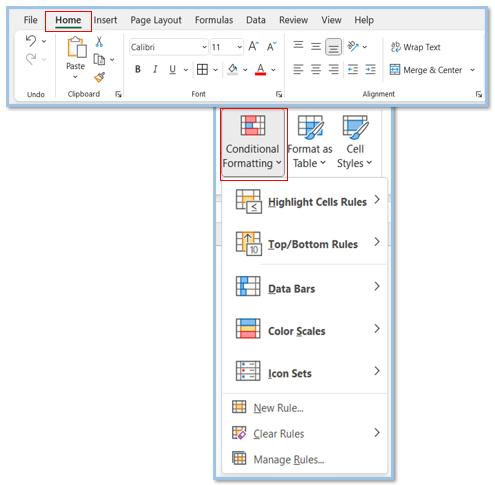
Highlight cells based on certain value/text
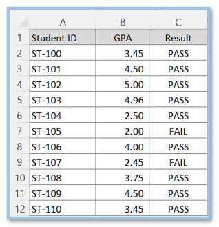
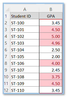
Highlight cells that have GPA of 3.50 and higher
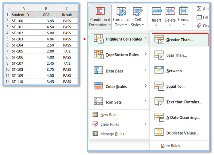
Step 1: Select the GPA column i.e. Col B and select the Highlight Cells Rules then Select Greater Than…
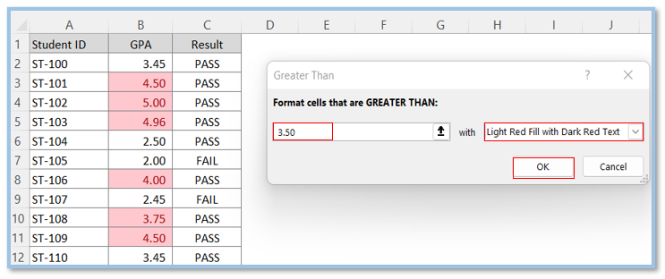
Step 2: Follow the next step to highlight GPA values greater than 3.50
How to clear or remove conditional formatting?
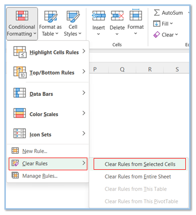
Step 1: Select range from B2:B12
Step 2: Select ‘Clear Rules’ and then select Clear Rules from Selected Cells. You may choose to remove the conditional formatting from the entire sheet by selecting the second option.
Highlight a Text
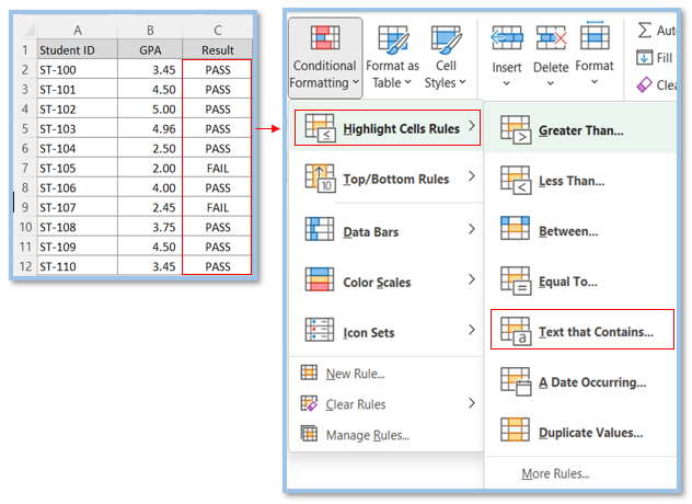
Highlight here all FAIL from the Result column.
Step 1: Select the Result column i.e. Col C and then select the ‘Text that Contains….’ rule
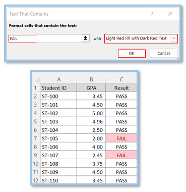
Step 2: Type Fail in the box shown below and select Light Red Fill with Dark Red Text from the other box and click OK.
Find the Duplicate value i.e. same GPA number appears multiple times
Step 1: Select column B and click on Duplicate Values.
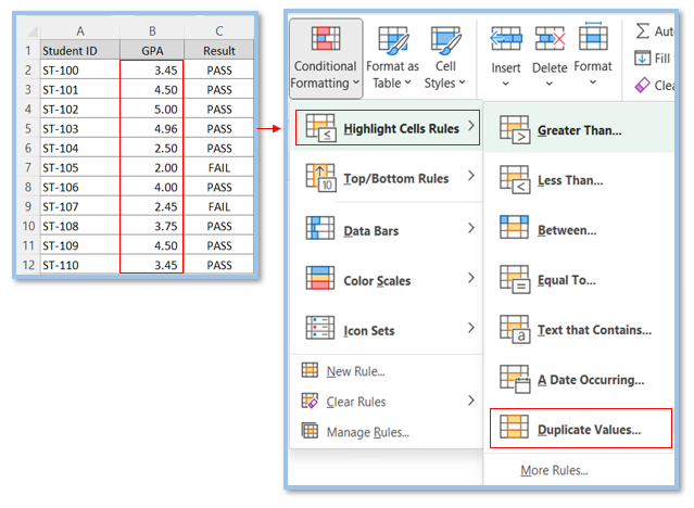
Step 2: Follow the steps as shown in the picture below.
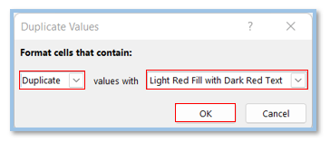
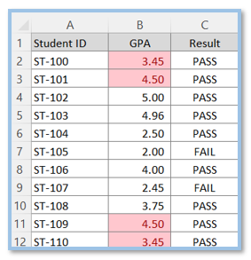
Step 3: Here GPA 3.45 and 4.50 appeared multiple times and were highlighted in dark red.
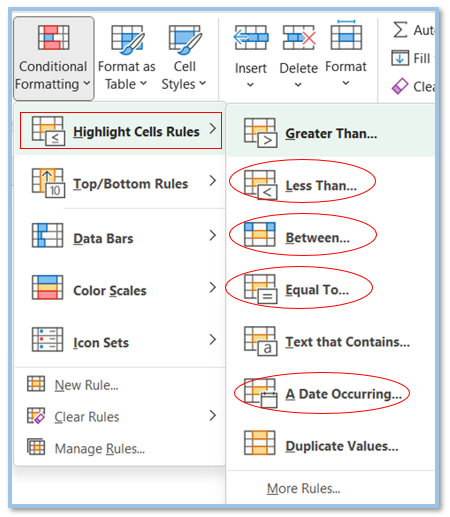
You can play around with other Cell Highlighting Rules
Highlight Top/Bottom 10 (10%)
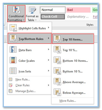
Step 1: Select the column you want to highlight, click on Top/Bottom Rules and then access the Top 10 Items (or%) / Bottom 10 Items (or%).
Step 2: The dialogue box will open depending on what you choose. Suppose you clicked on the Top 10 Items; a dialogue box would then appear. Now follow the steps below and click OK.
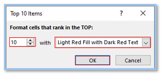
This only functions for cells that contain a numeric value. If you choose to highlight the Top 10 items or the Bottom 10 Items in a dataset with fewer than 10 cells, all of the cells will be highlighted.
Highlight Errors/Blanks
You can easily locate and highlight cells that contain mistakes or are empty by using conditional formatting in Excel.
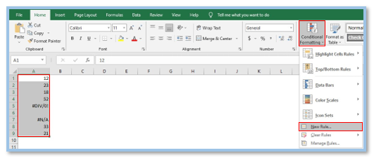
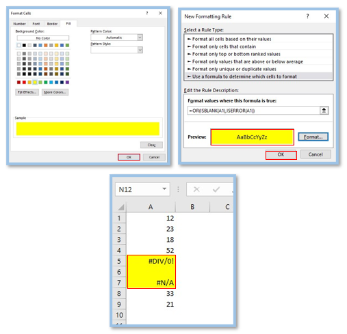
Let’s say we have the dataset as displayed below which has a blank cell (A6) and errors (A5 & A7)
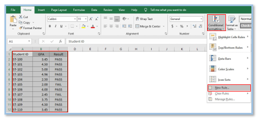
Step 1: Select column A, and click on Conditional Formatting >> New Rule.
Step 2: Select Use a formula to determine which cells to format and in the area labeled “Edit the Rule Description,” enter the formula shown below. Now click of Format.
=OR(ISBLANK(A1),ISERROR(A1))
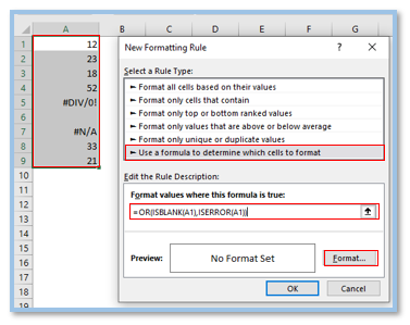
Step 3: To highlight blank or incorrect cells, choose your desired format and click OK. All the cells that are empty or contain errors would be instantly highlighted.
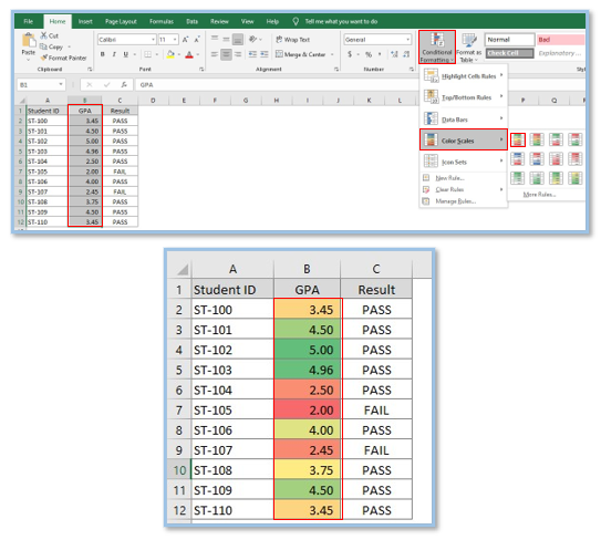
Creating Heat Map
A heat map can be made, with the cell with the greatest value being colored green and the color shifting from green to red as the value lowers. Values in the GPA column range from 2 to 5. Green is assigned to 5 while red is assigned to 2.
Select the GPA column and click Conditional Formatting >> Color Scales and chose one of the color schemes. Immediately the formatting will be applied in your datasheet.
Highlight Every Other Row Column
To highlight every other row and columns, follow the steps below.
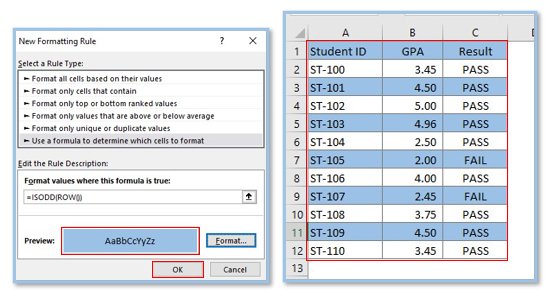
Step 1: Select A2-C12 and click on Conditional Formatting >> New Rule.
Step 2: Select Use a formula to determine which cells to format and in the area labeled “Edit the Rule Description,” enter the formula shown below. Now click of Format.
=ISODD(ROW())
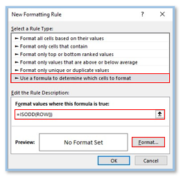
Step 3: Choose your desired format and click OK. It will highlight the alternate rows in the data set.
A similar method may be applied in several situations. Simply apply the appropriate formula in the conditional formatting. Here are a few instances:
=ISEVEN(ROW()) highlights alternate even rows.
=ISODD(ROW()) will be used to highlight alternative add rows.
=MOD(ROW(),3)=0 will be used to highlight each third row.
The various conditional formatting methods in Excel that visually improve the presentation of a dataset include data bars, color scale, and icon sets. In these methods, data is represented by bars, color combinations, icons etc.
Apply Data Bars Conditional Formatting
Follow the steps bellow for applying data bars conditional formatting.
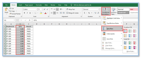
Step 1: Select GPA column and click on Conditional Formatting >> Data Bars and select any of the Gradient Fill.
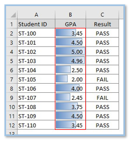
Step 2: Data bar is applied on the selected column’s data.
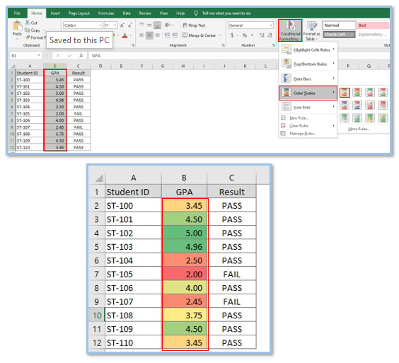
Apply Color Scales Conditional Formatting
Follow Step 1 from Apply Data Bars and then click on Color Scale and chose any of the color scale you want. It will immediately be applied to your worksheet data.
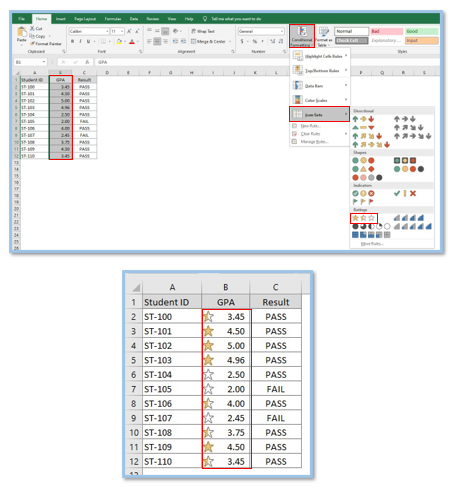
Apply Icon Sets Conditional Formatting
Follow Step 1 from Apply Data Bars and then click on Icon Sets and chose any sets of icons you want based on the data on your worksheet. It will immediately be applied to your worksheet data.
Application of Conditional Formatting in Excel
- Highlighting important data: Use conditional formatting to emphasize key information in your spreadsheet, such as highlighting cells with values above or below a certain threshold.
- Data validation: Apply conditional formatting to validate data entries, ensuring they meet specific criteria or constraints set by your business rules.
- Identifying trends: Utilize color scales or icon sets to visually identify trends or patterns in your data, making it easier to spot highs, lows, or changes over time.
- Error checking: Set up conditional formatting rules to automatically flag potential errors or inconsistencies in your dataset, helping you maintain data accuracy.
- Prioritizing tasks: Assign different colors or formats to tasks based on their priority level, allowing you to focus on high-priority items and manage your workload effectively.
- Custom formatting: Create custom conditional formatting rules to suit your specific needs, such as highlighting duplicate values, unique values, or cells containing specific text.
For ready-to-use Dashboard Templates:
