INDEX and MATCH functions in Excel are powerful tools for performing lookups and retrieving data from a table or range. Excel is a powerful tool that offers a wide range of functions to help us manipulate and analyze data effectively. Among these functions, INDEX and MATCH stand out as a dynamic duo, capable of performing complex lookups and retrieving specific information from large datasets. Whether you’re a beginner or an experienced Excel user, mastering the INDEX and MATCH functions can significantly enhance your data analysis skills.
This Tutorial Covers:
- The Basics of INDEX and MATCH Function
- INDEX Function
- MATCH Function
- INDEX and MATCH Function Together
- How to Use INDEX and MATCH Function in Excel
- Two-way lookup
- Left lookup
- Case-sensitive lookup
- Closest Match
- Multiple criteria lookup
- INDEX MATCH with MAX, MIN and AVERAGE
- INDEX MATCH with IFNA / IFERROR
- INDEX MATCH vs VLOOKUP
1. The Basics of INDEX and MATCH Function
1.1 INDEX Function
You’ll find the Excel INDEX function in a vast variety of calculations, especially complex formulas. It is highly customizable and powerful. A value at a designated area in a range can be obtained via INDEX.
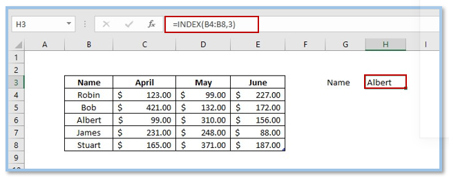
Below you have a table which contains the name list of 5 salesmen. Now use the formula below
to get the name of the 3rd salesman.
=INDEX(B4:B8,3)
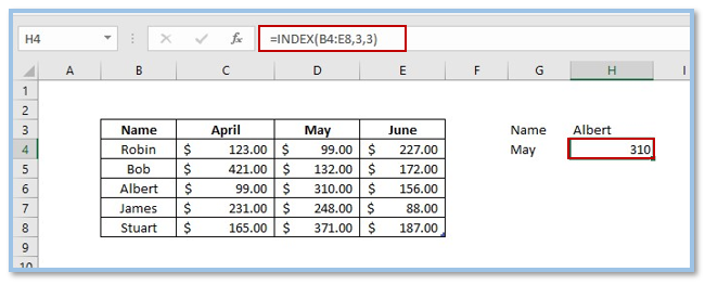
You can also retrieve the information about the sales status for 3rd salesman in May using the rows and columns information in Index formula.
=INDEX(B4:E8,3,3)
1.2 MATCH Function
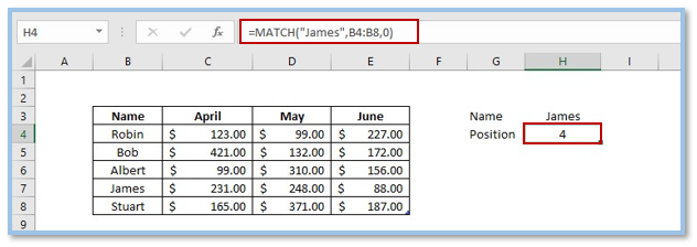
Finding an item’s location in a range is the only thing the MATCH function is intended to do. The location of a value inside a specified range is returned by the MATCH function. Using the Match function, you can acquire data about any salesman’s position on the spreadsheet.
=MATCH(“James”,B4:B8,0)
1.3 INDEX and MATCH Function Together
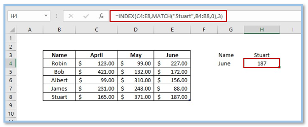
Using the Index function, you have gathered the information about the 3rd seller Albert and how much he sold in February using the data from both row and column. The Match function provided you with information about a particular seller’s serial number. Now you can very easily combine Index and Match function in a single formula and gather the information about how much the 5th seller sold in June following the picture below.
=INDEX(C4:E8,MATCH(“Stuart”,B4:B8,0),3)
Also Read: How to use XLOOKUP in Excel?
2. How to Use INDEX and MATCH Functions in Excel
In this tutorial, we have seen how the Index and Match function work separately and how can we combine them in a single formula to make our work easier and quicker. There are a variety of uses of the Index Match function in Excel. Now we will learn about the uses of the Index and Match Functions in a detailed manner.
2.1 Two-way lookup
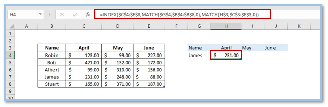
Using Index and Match we can execute a Two-Way lookup. From the table below you can acquire information about any seller’s sell data of April, May and June. Here you will use the 4th seller James and gather his sells data for these three months.
Step 1: Type or paste the formula in cell H4 and click Enter. You will get the sells data of James from April.
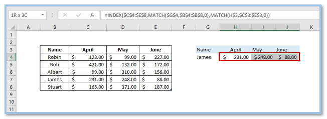
Step 2: Now paste the formula in the other two cells under May and June or simply just drag the data from H4 to J4 to get the sales data of the other two months using the same Index and Match formula.
The Index formula here used from cell C4 to E8 as a range that has all the sales data from each month of every seller and the first MATCH retrieves the name’s location in the name’s column using the name (James in cell G4) (B4:B8).
The month name (in cell H3) is used in the second MATCH formula to determine where that particular subject name is located in the range C3:E3. For instance, April ranks first, May second, and June third. Since the INDEX function receives these MATCH locations as input, it outputs the score based on the seller’s name and month name. Now if you want to know the data of any other seller simply just type the name of that seller instead of James in cell G4.
2.2 Left lookup
The capability of performing a “left lookup” is one of the primary advantages of INDEX and MATCH function. Using Index and Match function you can retrieve the total sales data for any particular seller while the sale data is on the left of the seller.
Select the cell below Bob’s Total sale and type or paste the formula shown in the picture. Click Enter.
=INDEX($B$4:$C$8,MATCH(“Bob”,C4:C8,0),1)
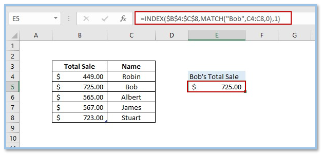
The Index formula uses from cell B4 to C8 as it’s range. The Match formula uses the name Bob to locate its location in range C4 to C8 to retrieve Bob’s sales data from Total sale’s column.
2.3 Case-sensitive lookup
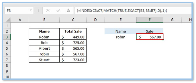
The MATCH function is not case-sensitive on its own. But, to execute a lookup that takes into account both upper- and lowercase letters, you can combine the EXACT function with INDEX and MATCH. When there is a chance of repetition or distinct names in huge data sets, with the case being a major distinction, you have to apply this method to get your desired data.
Step 1: Select the cell under Sale and type or paste the formula shown in the picture.
=INDEX(C3:C7,MATCH(TRUE,EXACT(E3,B3:B7),0),1)
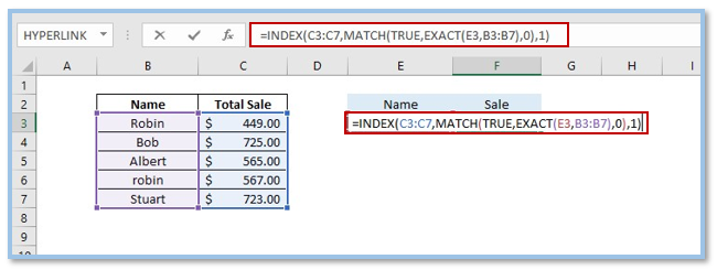
Step 2: Use CTRL+SHIFT+ENTER command key to because this is an array formula and only Enter will not work here.
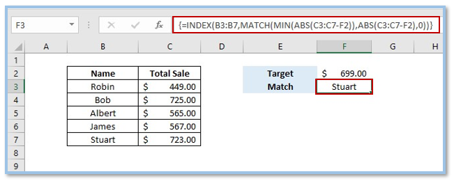
2.4 Closest Match
Use the Excel functions INDEX, MATCH, ABS, and MIN to discover the data in a column that matches a target value the closest.
Use the below-given formula in the cell under the target value and use CTRL+SHIFT+ENTER command key to because this is an array formula. By this method, you can extract the closest match to your target value.
=INDEX(B3:B7,MATCH(MIN(ABS(C3:C7-F2)),ABS(C3:C7-F2),0))
Also Read: How to a Picture Lookup in Excel?
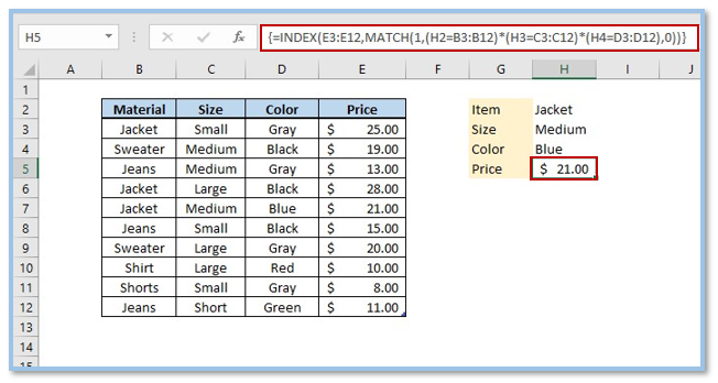
2.5 Multiple criteria lookup
A lookup, based on multiple criteria is among the toughest issues in Excel. In other words, a search that simultaneously matches values from many columns is a very complicated issue while using the Index Match function. But by utilizing INDEX, MATCH, and Boolean logic it is possible to derive data from these types of columns.
Use the following formula in the cell on the right of Price and Use CTRL+SHIFT+ENTER command key. This will show you the price of your desired item.
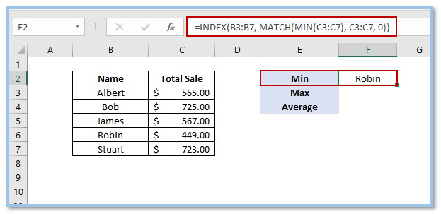
2.6 INDEX MATCH with MAX, MIN, and AVERAGE
In order to identify the minimum, maximum, and average values inside a range, Microsoft Excel provides unique functions. You can execute this by combining INDEX MATCH with the MAX, MIN, or AVERAGE functions.
Step 1: To find out the minimum amount from the Total sales column and who made the lowest sales, use the combined formula of INDEX MATCH and MIN and click Enter.
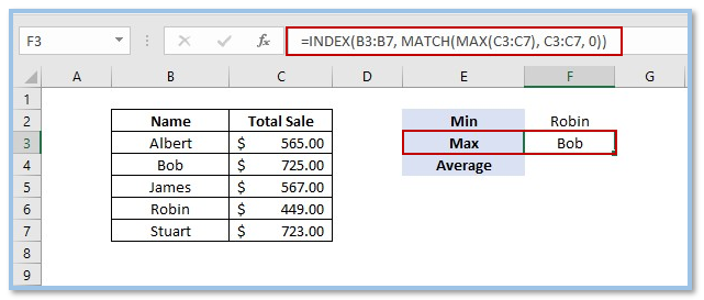
Step 2: Use the combined formula of INDEX MATCH and MAX and press Enter to determine the maximum amount from the Total sales column and who made the highest sales.
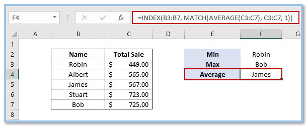
Step 3: Use the combined INDEX MATCH and AVERAGE formula and press Enter to determine the average of Total sales as well as the seller who made the average sales.
2.7 INDEX MATCH with IFNA / IFERROR
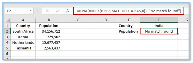
Step 1: Excel’s INDEX MATCH formula generates a #N/A error if it is unable to locate a lookup value. Wrap your INDEX MATCH formula in the IFNA function if you want to replace the usual error notation with something more relevant.
=IFNA(INDEX(B2:B5,MATCH(F1,A2:A5,0)), “No match found”)
Use the IFERROR function rather than IFNA if you want to capture all errors instead of just #N/A.
= IFERROR(INDEX(B2:B5,MATCH(F1,A2:A5,0)), “ Oops, something went wrong! “)
3. INDEX MATCH vs VLOOKUP
INDEX MATCH function and VLOOKUP both are very useful while retrieving complex data from a worksheet. Here you will see a brief comparison between both options for your better judgment in deciding which method to use to make your work more efficient and less time-consuming.
- The first disadvantage of VLOOKUP is that it can’t look to its left so the table’s leftmost column should always contain your lookup value. On the other hand, INDEZ MATCH can do it very efficiently.
- The only viable option if your dataset contains lengthy strings is INDEX MATCH because the total number of characters in your search criteria cannot exceed 255 when using the VLOOKUP function; otherwise, the #VALUE! The error will occur.
- MATCH INDEX will perform significantly more quickly than VLOOKUP if your worksheets include hundreds or thousands of rows, and consequently hundreds or thousands of formulas since Excel will only need to process the lookup and return columns rather than the complete table array.
- If your worksheet contains sophisticated array formulae like VLOOKUP and SUM, the influence of VLOOKUP on Excel’s performance may be more apparent. This situation will require VLOOKUP Function and INDEZ MATCH won’t be of any use here.
- When a new column is removed from or added to a lookup table, VLOOKUP formulae become unusable or produce inaccurate results. On the other hand, you give the return column range rather than an index number when using INDEX MATCH. As a result, you are free to add and remove as many columns as you like without having to worry about modifying each formula that is connected with them.
For ready-to-use Dashboard Templates:
