The PMT function is a powerful tool in Microsoft Excel that allows users to calculate the periodic payment amount for a loan. Whether you’re planning to buy a car, purchase a house, or invest in a business venture, understanding how much you need to pay each period is essential. The PMT function takes into account factors such as the interest rate, loan duration, and principal amount to determine the regular payment required. By utilizing this function, Excel users can quickly and accurately calculate loan payment amounts, enabling informed financial planning and decision-making. In this article, we will explore the PMT function in Excel and provide step-by-step instructions on how to use it effectively for loan calculations.
This Tutorial Covers:
- What does Excel’s PMT function do?
- Excel’s PMT function syntax
- Excel PMT function argument
- Examples of PMT Operations
- Example 1: Determining the Monthly Loan Amount for a Home Mortgage
- Example 2: Monthly Payment to Increase Investment to $100,000
- Calculate payments for the week, the month, the quarter, and the half-year
- Ineffective PMT function in Excel
1. What does Excel’s PMT function do?
Using a constant interest rate, the number of repayment periods, and the loan sum, the Excel PMT function computes the loan payment.
PMT means for “payment,” thus the name of the function.
A PMT formula can estimate your monthly payments, for instance, if you are looking for a $10,000 home loan with a seven-year term and a 5% annual interest rate.
Please remember the following details so that your worksheets’ PMT feature operates properly:
- The payment amount output is a negative figure because it is a cash outflow, in keeping with the overall cash flow model.
- The PMT function returns a value that contains principal and interest but excludes any possible fees, taxes, or reserve payments that may be related to a loan.
- For various payment frequencies, such as weekly, monthly, quarterly, or yearly, an Excel PMT formula can calculate the debt payment. The proper method is demonstrated in this example.
In Excel for Office 365, Excel 2021, Excel 2019, Excel 2016, Excel 2013, Excel 2010, and Excel 2007, the PMT feature is accessible.
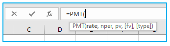
- Excel’s PMT function syntax:
The Excel PMT function code is listed below:
=PMT(rate, nper, pv, [fv], [type])
- Excel PMT function argument:
These parameters are available for the PMT function:
rate: It is the monthly interest amount that you must pay. For instance, rate/12 would apply if the installments were monthly. The rate will be rate/4 if it is quarterly.
nper: It is the quantity of repayment intervals for the loan.
pv: It is the loan’s present worth. This would be USD 10,000 in the case of the home loan above.
fv: [optional argument] After the loan is repaid, you want the potential value of your payments. If you only want to pay off the debt and nothing else, leave it out or change it to 0.
2. Examples of PMT Operations:
The periodic payment for a debt is returned by the Excel PMT function, which is a financial function. Given the loan sum, the number of repayment periods, and the interest rate, you can use the PMT function to calculate the loan’s payments.
Excel’s PMT feature has a wide range of applications.
Examples of its use are provided below.
- Example 1: Determining the Monthly Loan Amount for a Home Mortgage:
Assume you have a $10,000 home loan with a 7-year repayment period, a monthly payment schedule, and a 5% interest rate.
The arguments are described in more depth below:
rate – 5%/12 (since this the payment is monthly, you need to use the monthly rate) (since this the payment is monthly, you need to use the monthly rate).
nper – 7*12 (since the debt is to be paid for 7 years every month) (since the loan is to be paid for 7 years every month)
pv – $10,000 (this is the loan amount that I get today) (this is the loan value that I get today)
The optional parameters are not required and can be omitted.
How to use PMT function is shown below:
Step 1: Enter the following formula in cell B7 which utilizes the PMT function to determine the debt payment amount:
=PMT(B4,B5,B3)
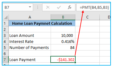
Due to the monetary outflow, the loan payment is negative. Make the loan sum negative if you want it to be positive.
Additionally, keep in mind that the interest rate will not change during the time period.
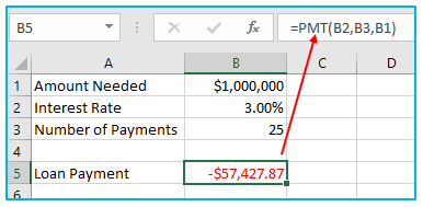
- Example 2: Monthly Payment to Increase Investment to $100,000:
The Excel PMT function can also be used to determine how much money you should set aside each month in order to receive a specific sum later on.
For instance, let’s say you want to make an investment that will yield $100,000 in 25 years at a 3% yearly interest rate.
The calculation’s method is as follows:
=PMT(B2,B3,B1)
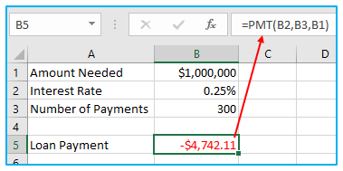
Due to the monthly installments, it should be noted that the interest is calculated as 3%/12.
If the installments are yearly, you can use an interest rate of 3%. (as shown below).
Also Read: How to Calculate Compound Interest in Excel
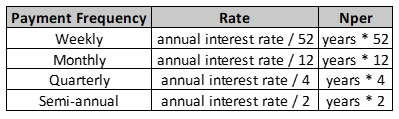
3. Calculate payments for the week, the month, the quarter, and the half-year:
You must perform the computations for the rate and nper arguments listed below depending on the payment frequency:
- For rate, by the number of yearly payments, divide the annual interest rate (which is deemed to be equal to the number of compounding periods).
- For nper, add the number of years and the annual contribution amount.
Details are provided in the chart below:
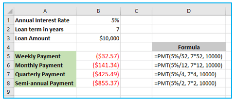
Use one of the formulas below to determine the amount of a periodic payment, for example, on a $10,000 loan with a 7-year term and a 5% yearly interest rate.
Weekly payment:
=PMT(5%/52, 7*52, 10000)
Monthly payment:
=PMT(5%/12, 7*12, 10000)
Quarterly payment:
=PMT(5%/4, 7*4, 10000)
Semi-annual payment:
=PMT(5%/2, 7*2, 10000)
The payments are always due at the end of each month, with the balance remaining after the final payment always being assumed to be $0.
The output of these algorithms is displayed in the screenshot below:
Also Read: How to Calculate Internal Rate of Return in Excel?
4. Ineffective PMT function in Excel:
If your PMT formula in Excel is malfunctioning or returning inaccurate data, one of the following is probably to blame:
- If either the rate argument is a negative integer or nper equals 0, a #NUM! error might appear.
- If one or more inputs are text values, a #VALUE! error is raised.
- Make sure you are consistent with the units provided for the rate and nper arguments if the output of a PMT formula is significantly higher or lower than anticipated. This means that you have correctly converted the annual interest rate to the period’s rate and the number of years to weeks, months, or quarters as shown above.
This is how the PMT formula in Excel is calculated.
For ready-to-use Dashboard Templates:
