Compound Interest in Excel is a powerful tool for financial planning and analysis. By harnessing the capabilities of Excel, users can accurately calculate compound interest for various financial scenarios, including loans, investments, and savings accounts. With its versatility and ease of use, Compound Interest in Excel empowers individuals and businesses to make informed decisions about their finances. Whether it’s planning for retirement, estimating loan repayments, or evaluating investment opportunities, Excel provides the flexibility and precision needed to navigate complex financial landscapes. With Compound Interest in Excel, users can unlock the potential of their financial data to achieve their goals and secure their financial future.
Compound Interest Excel Formula
It is easy to calculate compound interest in Excel. The formula for compound interest is FV = PV(1+r) n, PV stands for current value, FV for future value, r for interest rate per period, and n for the number of compounding periods.
What is compound interest?
Compound interest is when a loan, deposit, or interest earned on interest has interest added on top of the principal amount. Instead of being paid out, it is the result of reinvesting interest such that interest is received on the principal amount plus accrued interest over the subsequent period.
Consider investing $7,000 at a 10% yearly interest rate with annual compounding. In this case, you could receive $700 ($7,000 x 10%) as interest on your initial investment (principal). You may therefore make $7,700 from the first investment after earning $7,000 and $700. Then, based on the gross amount from the previous period, you may earn interest in the next period. In this example, if you invested $7,700 at the beginning, you may gain $770 ($7,700 x 10%) after two years. Your investment is now worth $8,470 ($7,700 + $770).
What is simple interest?
Simple interest is a simple and straightforward formula for figuring out how much interest will be charged on a loan. The daily interest rate, the principle, and the number of days between payments are calculated to calculate simple interest.
Although some mortgages employ this calculation approach, this kind of interest typically relates to auto loans or short-term loans.
Calculate Simple Interest
Take a look at an auto loan with a $15,000 principal balance and a 5% yearly simple interest rate to better understand how simple interest works. The finance business determines your interest on the 30 days in April if your payment is due on May 1 and you make it on time. In this case, your interest for 30 days is $61.64. The credit firm will only charge interest for 20 days in April if you make the payment on April 21, bringing your interest payment down to $41.09 and saving you $20.
How to calculate Compound Interest in Excel Formula (with example):
Using Mathematical Compound Interest Formula:
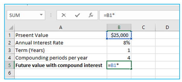
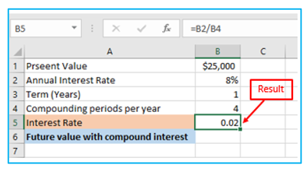
Step 1: Given that the principal amount is present in cell B1 (We can also call it as present value). This amount must be multiplied by the interest rate, outlined in Blue below.
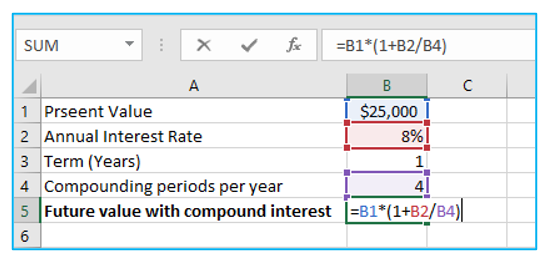
Step 2: We must divide the yearly interest rate by Cell B4 since the interest will be compounded quarterly (B4).
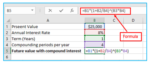
Step 3: Since interest is compounded four times per year, we must make a reference to a cell that contains the number of years in order to multiply 4 by that number. Because of this, the formula would be as follows, outlined in Red below.
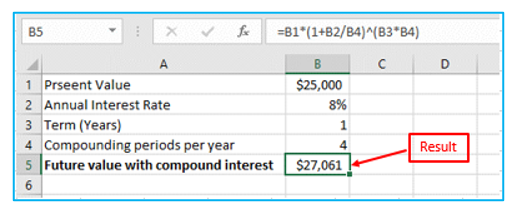
Step 4: After pressing the “Enter” button on the Keyboard, the result will show as follows, outlined in Red below.
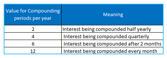
It is like a compound interest calculator excel formula now. You can also find compound interest formula excel monthly. The annual interest rate, the number of years, and the number of compounding periods per year can all be changed as shown below.
Also Read: How to Calculate Standard Deviation in Excel?
Using Compound Interest Calculation Table in Excel:
Procedure of calculating compound interest using compound interest calculation table as follows:
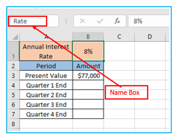
Step 1: Cell B1 needs to be selected, and its name needs to be changed to “Rate” using the “Name Box”, outlined in Red below.
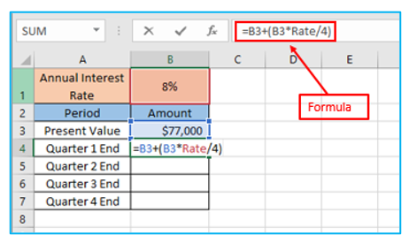
Step 2: With an 8% yearly interest rate, the principal value or present value is $77,000. We will multiply the principal amount by 8%/4, or 1.25% interest, to get the investment’s value at the conclusion of the first quarter. The formula is outlined in Red below.
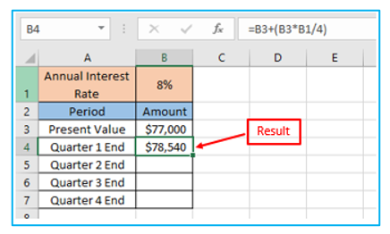
Step 3: After applying the formula, the result is shown below, outlined in Red below.
Step 4: After that, to fill all the cells, pull the “Fill Handle” further. The result is outlined in Blue below.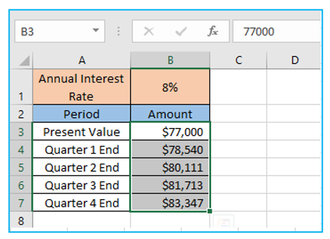
Compound Interest using FVSCHEDULE Excel Formula (Compound Interest Formula in Excel):
Procedure of calculating compound interest using FVSCHEDULE Excel Formula as follows:
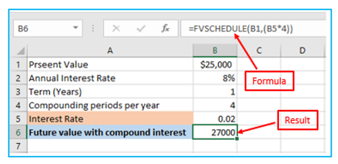
Step 1: We will enter the B1 cell reference for “primary” and 0.02 for “schedule,” respectively, because it is the result of dividing 8% by 4, outlined in Red below.
Step 2: After applying the FVSCHEDULE Formula in Cell B6, the result is shown in Red outline.
Several comments regarding the FVSCHEDULE Function:
- #VALUE! When one or more of the provided parameters is not a number, error will occur.
- Blank cells are accepted as a component of the scheduled array by the FVSCHEDULE function since they are viewed as the numeric value 0. They do not carry interest.
- Keep in mind that we must input the interest rates as an array of values if we enter them directly into the function rather than using cell references. FVSCHEDULE (B3, 0.025, 0.030, 0.040, 0.045), as a sample.
- We must use the FV function to calculate the future value of an investment if the interest rates are fixed and if we have access to the nper, pmt, and/or pv and type inputs.
Compound Interest using FV Excel Formula:
The FV function, which stands for Future Value, calculates an investment’s future value using periodic, constant payments and an interest rate that stays the same.
The FV function’s parameter is:
- Rate: In an annuity, rate refers to the fixed interest rate for each term.
- Nper: The total number of periods of an annuity is denoted by the term Nper.
- PMT: PMT signifies payment. It shows how much money we’ll put into the annuity each period. PV must be mentioned if this value is left out.
- PV: Present value is referred to as PV. It refers to the sum that we are investing. By convention, this amount is stated with a negative sign because it is money that we are spending out of our own pockets.
- Type: This parameter is optional. If the money is already being given to the investment at the end of the period we must indicate 0; if it is being added at the beginning of the period, we must specify 1.
Either the PMT or PV case must be brought up.
Also Read: How to Calculate Internal Rate of Return in Excel?
How to calculate the compound interest using FV Excel Formula on excel?
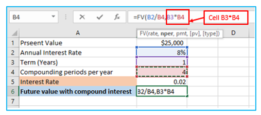
Step 1: FV stands for Future Value. In this example, FV Formula will be used in cell B6. “Annual Interest Rate (B2)/Compounding periods per year (B4)” will be used to determine the rate, outlined in Red below.
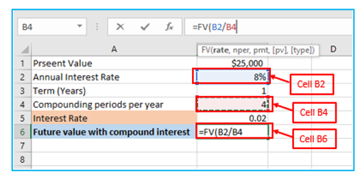
Step 2: The value of nper must be defined as “Term (Years) * Compounding periods per year”, outlined in Red below.
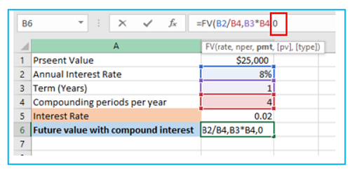
Step 3: We will enter “0” for “pmt” because there will be no extra principle value increments made between investing periods, outlined in Red below.
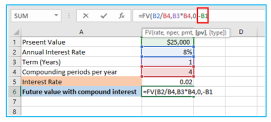
Step 4: The value for “pmt” has been eliminated, and the initial investment is worth $25,000 (present value). We’ll use the B1 cell with a “PV” reference that has a negative sign, outlined in Red below.
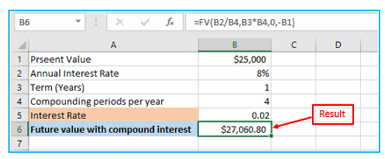
Step 5: After hitting the “Enter” button on the keyboard, we will get the result as the future value with compound interest, outlined in Red below.
Things to bear in mind when using the Compound Interest Formula for Excel:
- The interest rate must be entered in either decimal or percentage form, which is 4%. (0.04).
- In actuality, we need to specify the “PMT” and “PV” inputs in the FV function in the negative form (with a minus (-) sign).
- The FV function returns #VALUE. Any non-numeric value provided as an argument will result in an error.
- Either PMT or PV inputs must be mentioned in the FV function.
Application of Compound Interest in Excel
- Financial Planning: Calculate future savings or investment values based on compound interest, aiding in long-term financial planning.
- Loan Repayment: Determine the total interest paid over the life of a loan or mortgage, assisting in budgeting and debt management.
- Investment Analysis: Evaluate potential returns on investments by projecting compound interest growth over time.
- Retirement Planning: Estimate retirement savings growth to ensure sufficient funds are available for retirement years.
- Education Savings: Plan for future education expenses by projecting compound interest growth on college savings accounts.
- Debt Consolidation: Compare interest savings between different debt consolidation options to make informed decisions.
For ready-to-use Dashboard Templates:
