The Weighted Average Formula in Excel is your key to precision in calculations that demand a nuanced approach. This versatile tool allows you to assign weights to data points, ensuring that critical factors receive the attention they deserve. With ‘Weighted Average Formula in Excel,’ you’re not merely calculating averages; you’re making informed decisions based on weighted importance. Whether you’re evaluating student performance, financial metrics, inventory costs, or product ratings, this formula empowers you to extract meaningful insights and drive data-driven outcomes. Embrace the simplicity and impact of this function to elevate your Excel capabilities, making your worksheets a testament to meticulous analysis and informed decision-making. ‘Weighted Average Formula in Excel’ is your ally in achieving precision and relevance in your data calculations.
This Tutorial Covers:
- Excel formula for calculating weighted average
- SUMPRODUCT Function: Excel Weighted Average Calculation
- Example 1 – When the Weights Add Up to 100%
- Example 2: When the weights don’t total 100%
- Example 3: When It Is Necessary to Calculate the Weights
- SUM Function: Excel Weighted Average Calculation
- SUMPRODUCT Function: Excel Weighted Average Calculation
1. Excel formula for calculating weighted average
A weighted average is a type of arithmetic mean where certain data set components are given more weight than others. In other words, a certain weight is allocated to each number that will be averaged.
Weighted Formula Excel has Two types—the SUM function and the SUMPRODUCT function—will be used to determine the weighted average. Let’s go over each function individually.
- SUMPRODUCT Function: Excel Weighted Average Calculation:
There may be a number of situations when you need to compute the weighted average
Here are three such scenarios where you can utilize Excel’s SUMPRODUCT function to determine the weighted average in Excel.
- Example 1 – When the Weights Add Up to 100%
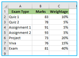
- Assume you have a dataset with a student’s grades from various tests as well as the weights in percentages, as shown below:
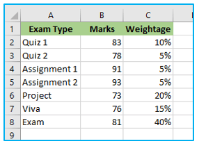
In the data above, a student receives points in several assessments, but ultimately needs to be awarded a grade or final score. Since the weights of the various evaluations vary, a simple average cannot be determined in this situation.
For instance, a quiz with a 10% weight has twice as much weight as an assignment, but only one-fourth as much weight as the test.
You can use the SUMPRODUCT function to obtain the weighted average of the score in this situation.
The Excel formula to calculate the weighted average is as follows:
=SUMPRODUCT(B2:B8,C2:C8)
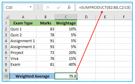
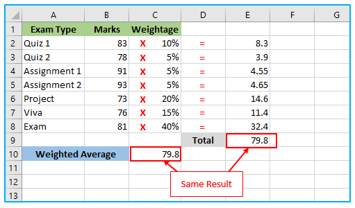
This formula works as follows: The first element of the first array is multiplied by the first member of the second array using the SUMPRODUCT function in Excel. The second element of the first array is then multiplied by the second member of the second array. so forth. It adds all of these values at the end.
Here is an example to help you understand.
- Example 2: When the weights don’t total 100%
In the situation mentioned above, the weights were set so that the sum totaled up to 100 percent. However, this might not always be the case in real-world circumstances.
Let’s examine the same scenario with various weights.
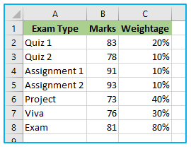
The weights in the aforementioned situation add up to 200%.
I will get the incorrect answer if I use the same SUMPRODUCT formula.
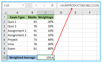
I have doubled all the weights in the result above, giving the weighted average of 159.6. Now that we know, no matter how brilliant a student is, he or she cannot receive more than 100 out of 100.
The weights don’t add up to 100%, which is the cause of this.
The equation for obtaining this is as follows:
=SUMPRODUCT(B2:B8,C2:C8)/SUM(C2:C8)
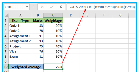
The SUMPRODUCT result is divided by the total weights in the calculation above. So, the weights would always add up to 100%, no matter what.
Also Read: How to Calculate Compound Interest in Excel
- Example 3: When It Is Necessary to Calculate the Weights:
The weights were specified in the previously discussed case. The weights may not always be readily available, in which case you must first determine the weights before determining the weighted average.
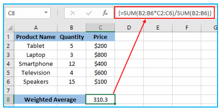
Assume you sell the following five different sorts of products:
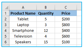
The SUMPRODUCT function can be used to determine the weighted average price for each product. The formula is as follows:
=SUMPRODUCT(B2:B6,C2:C6)/SUM(B2:B6)
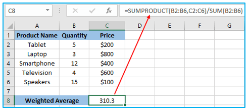
In order to ensure that the weights (in this example, the quantities) sum up to 100%, divide the SUMPRODUCT result by the SUM of the quantities.
- SUM Function: Excel Weighted Average Calculation:
The SUM function can also be used to calculate the weighted average in Excel, though the SUMPRODUCT formula Excel is recommended.
Each element’s percentage importance must be multiplied in order to compute the weighted average using the SUM formula Excel.
Using the similar dataset:
The equation that will provide the desired outcome is as follows:
=SUM(B2*C2,B3*C3,B4*C4,B5*C5,B6*C6,B7*C7,B8*C8)
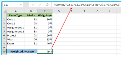
When you only have a few objects, you can use this strategy. However, this procedure could be laborious and prone to mistakes if you have a lot of products and weights. The SUM function can be used to complete this task faster and more effectively.
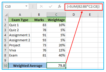
Using the same set of data, the following quick calculation will provide you with the weighted average using the SUM function:
=SUM(B2:B8*C2:C8)
When applying this formula, the secret is to use Control + Shift + Enter rather than just Enter. You must use Control + Shift + Enter to handle arrays because the SUM function cannot.
Also Read: How to Calculate Standard Deviation in Excel?
At the start and end of the formula, curly braces would automatically emerge when you pressed Control + Shift + Enter (see the formula bar in the above image).
Once more, confirm that the weights total up to 100%. If not, you must divide the outcome by the total of the weights (using the product example below):
Application of Weighted Average Formula in Excel
- Grades Calculation:
- Calculate a student’s final grade by assigning different weights to individual assignments, quizzes, and exams.
- Financial Analysis:
- Determine the weighted average cost of capital (WACC) by assigning weights to the cost of debt and cost of equity in a company’s capital structure.
- Inventory Valuation:
- Calculate the weighted average cost of inventory items to determine the cost of goods sold (COGS) and ending inventory.
- Product Ratings:
- Calculate a weighted average rating for products or services by assigning different weights to customer reviews based on their importance.
- Employee Performance:
- Evaluate employee performance by calculating a weighted average of various performance metrics, such as sales numbers, customer satisfaction scores, and attendance records.
- Project Management:
- Determine the weighted average project completion time by assigning weights to different project tasks or milestones.
The weighted average formula in Excel is a versatile tool for calculating averages based on different criteria and can be applied to various fields, including education, finance, and business analysis.
For ready-to-use Dashboard Templates:
