Slicers in Excel revolutionize data analysis by offering an intuitive and interactive way to filter information. With their user-friendly interface and visual representation, Slicers empower users to explore data subsets effortlessly. Whether it’s creating dynamic dashboards or conducting multi-dimensional analysis, Slicers streamline the process, providing insights with just a few clicks. Their versatility and ease of use make Slicers a valuable tool for professionals across various industries. Incorporating Slicers in Excel enhances data visualization and decision-making, ultimately improving productivity and efficiency. Harness the power of Slicers in Excel to unlock the full potential of your data analysis endeavors.
This Content Covers:
- What Are Slicers in Excel?
- Benefits of Using Slicers in Excel
- How to Insert a Slicer to a Regular Table?
- How to Insert a Slicer to a PivotTable?
- How to use a Slicer?
- How to Customize a Slicer in Excel?
1. What Are Slicers in Excel?
Slicers in Excel are a tool that is used to filter the data according to our needs by slicing a portion of the data from the generated table using the Pivot Table option in Excel. Slicers aid in more than simply data filtering; they also make it easy for you to understand the information that is being gathered out and shown on the screen.
2. Benefits of Using Slicers in Excel
Slicers have been shown to offer several benefits and to simplify life while performing real-time data analysis in Excel. Below are a few of the most significant advantages.
- Excel’s slicers are helpful in protecting data security and integrity since the user only wants to remove the relevant information and avoid tampering with the real data.
- Slicers replace the time-consuming approach of manually filtering the data by making it simple and quick to obtain the needed information in a short amount of time.
- Both the Slicer formulas and other formulas are simple to copy or transfer to various tables.
3. How to Insert a Slicer to a Regular Table?
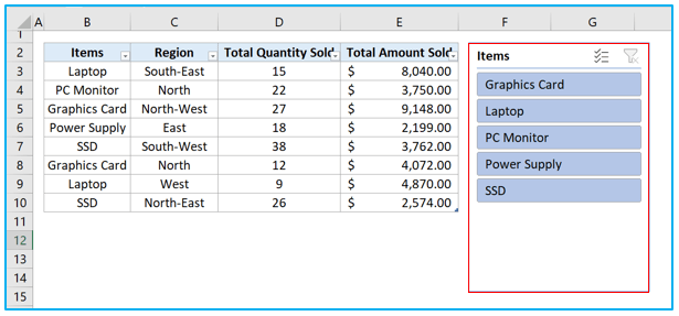
Suppose we have this tabular data in our Excel worksheet. Follow the step below to learn how to add or insert slicers to these sorts of regular tables in Excel.
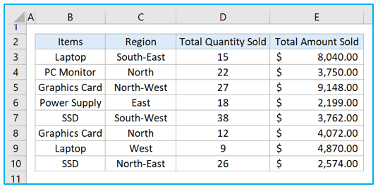
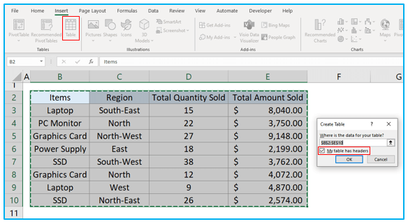
Step 1: Select the whole range or tabular data and press CTRL+T to open the Create Table dialogue box. Or you can go to Insert>>Table to create a table. Make sure My table has headers box is checked before clicking OK.
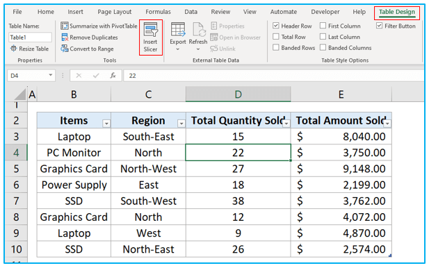
Step 2: After converting the tabular data into an actual table, select any cell from the table and go to Table Design tab. Click on the Insert Slicer option.
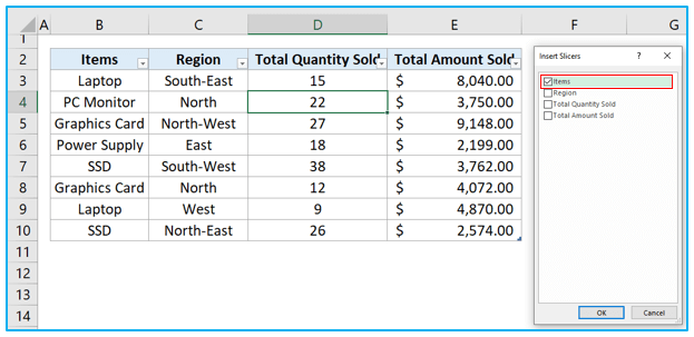
Step 3: The Insert Slicer box will open, select the required column title that you want to create a slicer of and press OK. Here the Items column has been selected to make a slicer of.
Step 4: When you press OK the selected slicer will be inserted inside your worksheet.
Also read: How to Add Calculated Field in Pivot Table?
4. How to Insert a Slicer to a PivotTable?
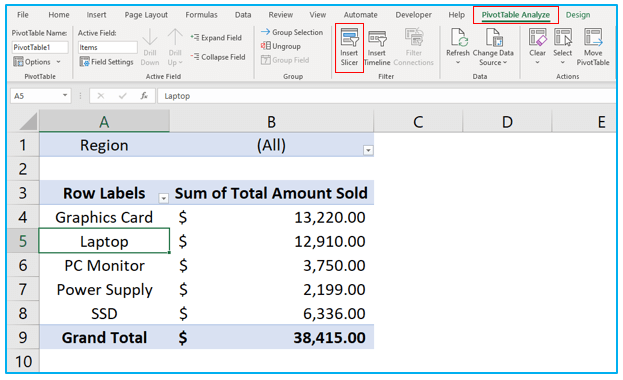
Step 1: To insert a slicer to a pivot table, select any cell from the table and go to PivotTable Analyze tab. Select Insert Slicer option.
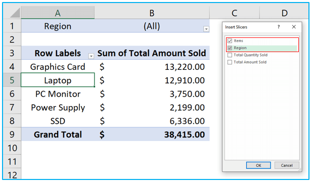
Step 2: Like the previous slicer insertion method, select the column titles and press OK.
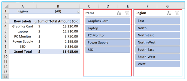
Step 3: The slicers have been inserted inside our worksheet.
Also read: How to Filter Data in Pivot Table in Excel?
5. How to use a Slicer?
After you have inserted a slicer, it’s time to learn how to use the slicer.
Step 1: There are two buttons inside a slicer,
- Multi-Select button
- Clear Filter button.
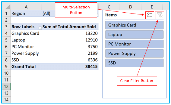
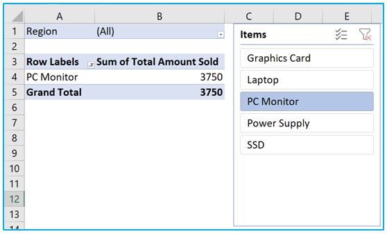
Step 2: If you want to select only one tab or one option inside the slicer and filter the data base on it, then click on any tab inside the slicer and the pivot table will be filtered according to it. When you click on another tab, the previous one gets deselected. Only one tab at a time can be selected in this way.
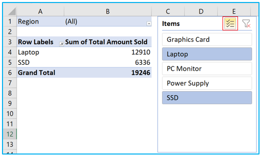
Step 3: If you want to select multiple tabs together, then click on the Multi-Select button. When its selected the button will glow like the picture below. Now click on the tabs that you want to select. If you want to reset the slicer, then click on the Clear Filter button.
6. How to Customize a Slicer in Excel?
There are various customizations available for a slicer. Let’s see how we can give our slicers a personal touch.
Step 1: Select the slicer and go to Slicer tab. From the Slicer Styles section, you can change the style and color of your slicer.
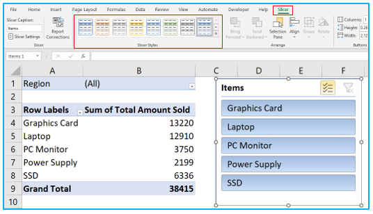
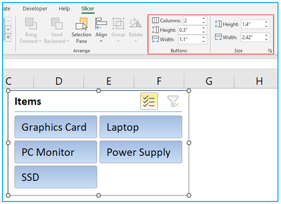
Step 2: From Button section you can select how many columns you want inside the slicer, and you can also change the height and weight of the buttons. Change the height and weight of the slicer from Size section.
Application of Slicers in Excel
- Data Filtering: Slicers provide an easy way to filter data in Excel tables or PivotTables, allowing users to quickly narrow down information based on specific criteria.
- Interactive Dashboard: Incorporating slicers into Excel dashboards enhances interactivity, enabling users to dynamically explore data subsets by selecting slicer options.
- Visual Representation: Slicers present filtering options in a visually appealing manner, making it easier for users to understand and interact with data.
- Multi-Dimensional Analysis: With slicers, users can perform multi-dimensional analysis by filtering data across multiple fields simultaneously, providing deeper insights into data relationships.
- Easy to Use: Slicers offer a user-friendly interface for filtering data without requiring complex formulas or advanced Excel skills, making them accessible to all users.
- Customization: Users can customize slicers by adjusting their size, appearance, and layout to suit their specific data visualization needs.
For ready-to-use Dashboard Templates:
