How to Filter Data in Pivot Table in Excel?

Filter Data in Pivot Table in Excel to revolutionize the way you analyze and interpret your datasets. This essential feature allows you to drill down into specific details, isolate key metrics, and remove unnecessary information, enabling a clearer, more focused analysis. Whether you’re aiming to understand customer demographics, track product performance, or manage financial budgets, filtering data in a pivot table provides the clarity and precision needed for informed decision-making. Harness the power of Excel’s filtering capabilities to transform overwhelming data into actionable insights and tailored reports.

This Tutorial Covers:

1. Filter types in a pivot table
2. Examples of Pivot Table Filters in Use
   • Filter a pivot table’s top 10 items
     • Filter Items at Top and Bottom by Value
     • Select Items at the Top and Bottom that Comprise a Specific Percent of the Value
     • Filter Items at the Top and Bottom That Comprise a Specified Value
   • Filter Items according to Value
   • Use Label Filters to Filter Data
   • Data Filtering via the Search Box

1. Filter types in a pivot table

Here is an example of the various filters that may be used with a pivot table.

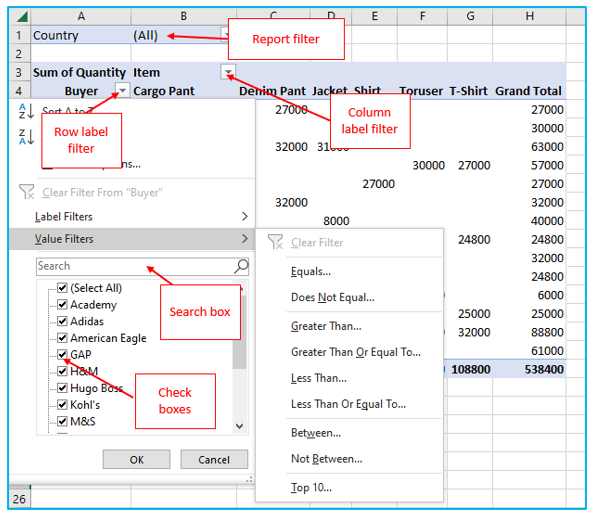
Let’s examine each of these filters separately:

Report Filter: This filter enables you to explore a portion of the complete dataset. For instance, if you have data on retail sales, you can examine the data by region by choosing one or more regions (yes, it allows multiple selections as well). Drag and drop the Pivot Table field into the Filters section to create this filter.

Row/Column Label Filter: With the help of these filters, you may narrow down the selection of pertinent data based on field values or field items (such as the top 10 things by value or items with a value more than/less than a particular value).

Search Box: You may easily filter using the text you provide by using this filter, which is accessible within the row/column label filter. For instance, if you only want data for Costco, enter Costco here, and the data will be filtered for you.

Checkboxes: These let you pick items from a list. For instance, you may do this here if you want to hand-pick retailers to study. Alternatively, you can uncheck it to specifically exclude selected retailers.

Here are some examples of how to utilize them in real-world settings to filter data in a pivot table.

2. Examples of Pivot Table Filters in Use

In this section, we’ll look at the following examples:

• Filter a pivot table’s top 10 items
• Filter Items according to Value
• Use Label Filters to Filter Data
• Data Filtering via the Search Box

Filter a pivot table’s top 10 items

The top 10 filter options in a pivot table can be used to:

• Filter Items at the Top and Bottom by Value.
• Select Items at the Top and Bottom that Comprise a Specific Percent of the Value.
• Filter Items at the Top and Bottom That Comprise a Specified Value.

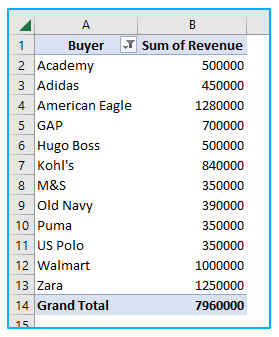
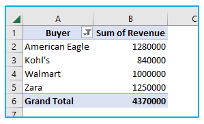
Assume you have the pivot table depicted below:

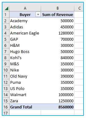
Let’s practice applying the Top 10 filter on this batch of data.

• Filter Items at Top and Bottom by Value

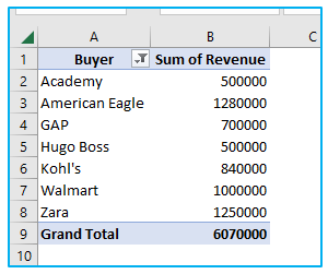
The Top 10 filter will provide you with a list of the top 10 buyers according to revenue worth.

The steps are as follows

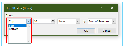
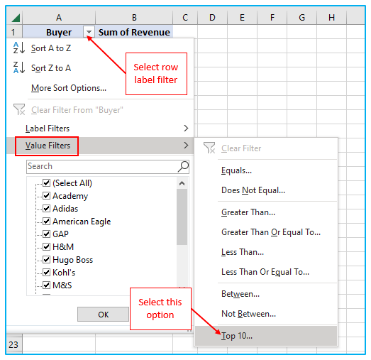
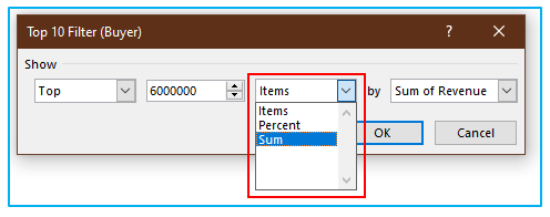
Step 1: Go to the Row Label filter in the pivot table. Then click “Value Filters” and then select “Top 10”.

 

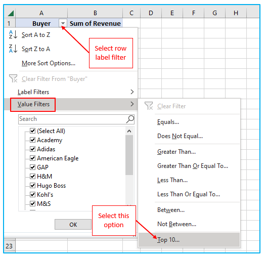
Step 2: There are four selections you must make in the “Top 10 Filter” dialog box:

• Top/Bottom: In this instance, choose Top as we’re seeking for the top 10 buyers.

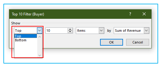
• How many items you wish to filter. Since we want the top 10 items in this situation, this would be number 10.

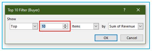
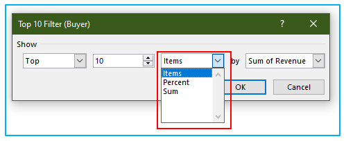
• Items, Percent, and Sum are the three possibilities in the drop-down menu in the third field. In this instance, choose Items since we want the top 10 buyers.

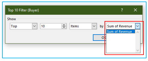
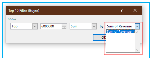
• All of the distinct values listed in the value area are listed in the final field. Since all we have in this situation is the sum of revenue, only “Sum of Revenue” is displayed.

You will receive a filtered list of 10 buyers based on the amount of their revenue from this.

The same method can be used to obtain the bottom 10 (or any other number) items in terms of value.

• Filter Items at the Top and Bottom that Comprise a Specific Percent of the Value

The top 10 filter allows you to obtain a list of the top 50% (or any other percentage, such as the top 20%, 30%, etc.) of items by value.

Let’s imagine you want to find out which buyers account for 50% of overall revenue.

The steps are as follows

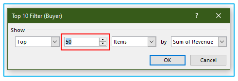
Step 1: Go to the Row Label filter in the pivot table. Then click “Value Filters” and then select “Top 10”.

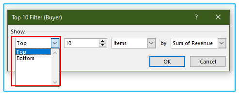
Step 2: You must choose one of four options in the “Top 10 Filter” dialog box:

• Top/Bottom: In this instance, choose Top since we are seeking for the top buyers that generate 50% of the total revenue.

• You must enter the percentage of revenue that should be accounted for by the top buyers in the second field. This would be 50 in this instance since we want to attract the top buyers who contribute 50% of the revenue.

• Go to the third field and choose Percent.

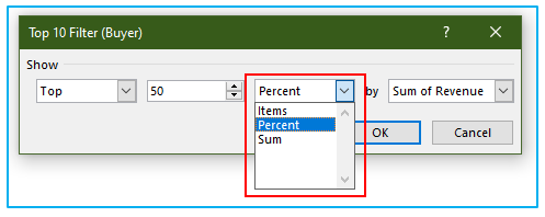
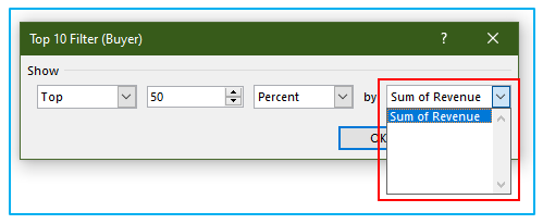
• All the distinct values listed in the value area are listed in the final field. In this instance, it merely says “Sum of Revenue” because all we have is the total revenue.

This will provide you with a list of buyers whose combined revenue account for 50% of the total.

The similar procedure can be used to identify the buyers who account for the bottom 50% (or any other proportion) of total revenue.

• Filter Items at the Top and Bottom That Comprise a Specified Value

Let’s imagine you want to identify the top buyers that contributed 6 million in revenue.

The Pivot Table’s Top 10 filter can be used to do this.

The steps are as follows

Step 1: Go to the Row Label filter in the pivot table. Then click “Value Filters” and then select “Top 10”.

Step 2: You must choose one of four options in the “Top 10 Filter” dialog box:

• Top/Bottom: In this instance, choose Top as we’re seeking for top buyers who generate 6 million in revenue overall.

• You must enter a value that the top buyers should take into account in the second field. This would be 6000000 in this instance since we are trying to obtain the top buyers that account for 6 million in revenue.

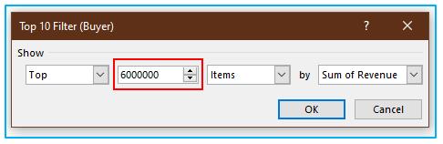
• Choose Sum in the third field.

• All of the distinct values listed in the value area are listed in the final field. In this instance, it merely says “Sum of Revenue” because all we have is the total revenue.

You will receive a list of the top buyers, who account for 6 million of the total revenue, after doing this.

• Filter Items according to Value

Based on the values in the columns in the values box, you can filter the items.

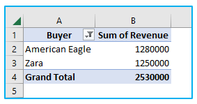
Assume you have the pivot table depicted below, which was made using buyer revenue data:

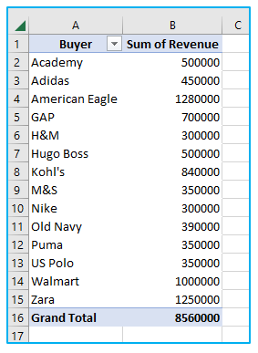
This list can be filtered according to revenue amount. Consider the scenario where you want a list of all the buyers with more than 1 million in revenue.

The steps are as follows

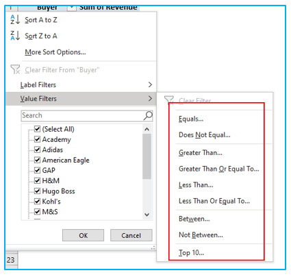
Step 1: Go to Row Label filter in the pivot table. Then click “Value Filters” and then select “Greater Than…”.

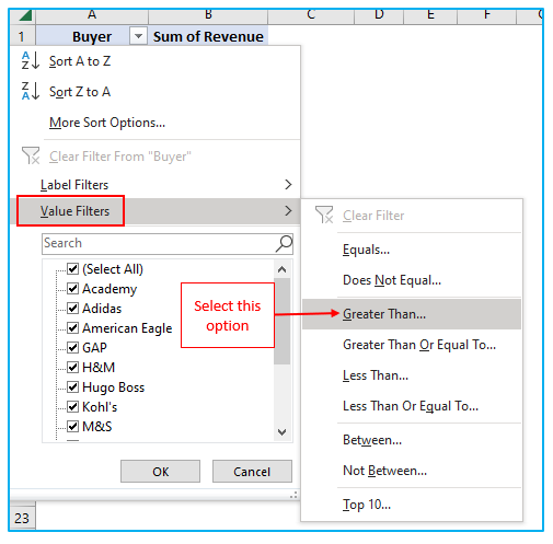
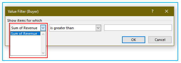
Step 2: The “Value Filter” dialog box contains:

Choose the values you want to apply as filters. It is the Sum of Revenue in this instance (if you have more items in the values area, the drop down would show all of it).

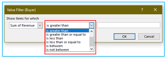
• Choose the circumstance. Select “is greater than” because we want to find any buyer with a revenue of more than 1 million.

• Fill out 1000000 in the final field. Select OK.

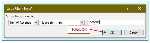
This would instantly filter the list and show only those buyers that have revenue more than 1 million.

Like this, you can use a variety of different conditions, including equal to, does not equal to, less than, between, etc.

• Use Label Filters to Filter Data

When you have a long list and wish to filter out some things based on their name or text, label filters come in handy.

For instance, by adding the criteria “Walmart” in the name, I can rapidly filter out all the Walmart locations from the list of buyers.

The steps are as follows

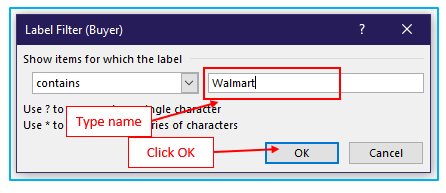
Step 1: Go to the Row Label filter in the pivot table. Then click “Label Filters” and then select “Contains…”.

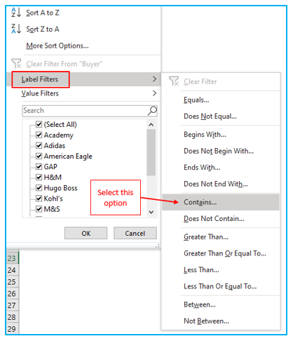
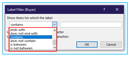
Step 2: In the dialog box for the “Label filter”:

‘Contains’ is the default choice (since we selected contains in the previous step). If you’d like, you can modify this right here.

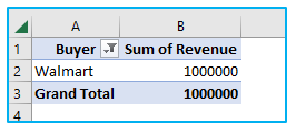
• If you wish to filter the list, enter the text string. It is “Walmart” in this instance. Select OK.

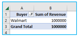
This would instantly filter the list and show only “Walmart” buyer.

Other label filters, such as begins with, finishes with, does not contain, etc., can be used in a similar manner.

• Data Filtering via the Search Box

The contains option in the label filter is quite similar to how you may filter a list using the search box.

For instance, typing Walmart into the search box will restrict the results to only show buyers with the word “Walmart” in their name.

the following steps:

Step 1: To put the cursor in the search box, first select the Label filter drop-down menu.

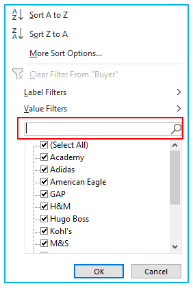
Step 2: Enter the search term, in this example “Walmart.” Below the search field, you’ll see that the list is filtered, and you can uncheck any other buyer you want to disregard. Select OK.

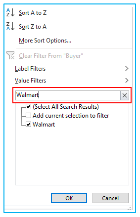
This would immediately filter out any buyers who used the word “Walmart.”

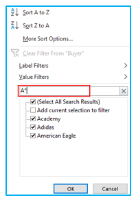
In the search field, wildcard characters are supported. Use the search query A*, for instance, to see all the purchasers whose names begin with the letter A. (A followed by an asterisk). The name can include any number of characters following A because an asterisk can represent any number of characters.

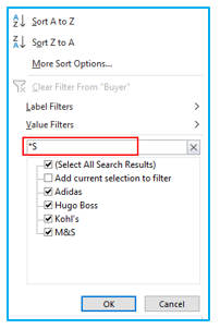
Similarly, if you want to get the list of all the buyers that end with the alphabet S, use the search term as *S (asterisk followed by S).

A few crucial details concerning the search bar are as follows:

• The first criterion is discarded, and you obtain a list of the second criteria if you filter once with one and then again with another. There is no additive filtering.
• You can manually deselect some of the results when using a search box. For instance, if you have a long list of financial institutions and want to solely filter out banks, you can search for “bank.” You may just uncheck it and keep it out if any businesses enter that are not banks, though.
• You cannot rule out particular outcomes. There is no option to use the search box to exclude only the merchants that have the word dollar in them, for instance. However, you may accomplish this by utilizing the label filter’s “does not contain” condition.

How ‘Filter Data in Pivot Table’ helps to improve the Dashboard Reporting?

Here are six key ways in which ‘Filtering Data in Pivot Tables’ enhances dashboard reporting:

1. Enhanced Data Relevance:By filtering data in pivot tables, you can remove irrelevant information, ensuring that your dashboard only displays data that is pertinent to your specific analysis or reporting needs. This leads to more focused and meaningful insights.
2. Improved Data Visualization:Filters help in simplifying complex data sets, making it easier to create clear and concise visualizations on your dashboard. This clarity is essential for quickly conveying key information to stakeholders who may not be familiar with the underlying data.
3. Dynamic Data Interaction:Pivot table filters allow for interactive dashboards. Users can select specific criteria or parameters to view customized data sets. This interactivity makes the dashboard more user-friendly and adaptable to different analytical requirements.
4. Time Efficiency:Filtering data directly within pivot tables speeds up the process of data analysis and reporting. Instead of manually sifting through large datasets, you can quickly display only the relevant data, saving significant time and effort.
5. Targeted Analysis:With the ability to filter data, you can perform targeted analysis by focusing on specific segments, time periods, or categories. This targeted approach helps in identifying trends, anomalies, and opportunities that might be missed in a broader analysis.
6. Comparative Analysis:Pivot table filters facilitate the comparison of different data sets within the same dashboard. For instance, you can compare performance across different time periods, regions, or product categories, which is invaluable for strategic planning and decision-making.

Application of Filter Data in Pivot Table in Excel

• Data Segmentation: Use the filter function in pivot tables to view specific subsets of data, such as sales by region or product type, helping to focus on particular areas of interest.
• Time Period Analysis: Apply date filters to analyze data over different time periods, such as monthly, quarterly, or yearly, enabling trend identification and temporal comparisons.
• Customer Demographics Analysis: Filter data based on demographic criteria like age, gender, or location to understand customer behavior and preferences better, aiding targeted marketing strategies.
• Product Performance Evaluation: Utilize filters to assess the performance of various products or services, identifying top performers and underperformers for strategic planning and inventory management.
• Expense Tracking: Apply filters to categorize and analyze expenses by type, department, or project, assisting in budget management and cost reduction efforts.
• Market Comparison: Use filters to compare data across different markets or segments, helping to identify opportunities for expansion or areas requiring improvement.

For ready-to-use Dashboard Templates:

1. 1. Financial Dashboards
   2. Sales Dashboards
   3. HR Dashboards
   4. Data Visualization Charts