How to use the Match Function in Excel

Match Function in Excel is an essential tool for data analysis and management, enabling precise and dynamic data retrieval and comparison. By mastering this function, you can streamline your workflows, enhance data integrity, and unlock deeper insights into your datasets. Whether you are performing complex lookups, creating dynamic ranges, or ensuring data consistency, the Match Function in Excel offers the flexibility and power needed to handle a wide array of data challenges. Embrace this function to elevate your Excel skills and turn data into actionable intelligence.

What is the MATCH function in Excel?
How to apply an Exact match?
Types of Match mode behavior information.
Apply Multiple criteria in Excel.
Apply Approximate match in Excel.

1. What is the MATCH function in Excel?

Matching functions in Excel are a group of functions designed to locate specific data within your spreadsheets based on defined criteria. They’re essential for data analysis, information retrieval, and creating dynamic formulas that adapt to changing data. Syntax: MATCH (lookup_value, lookup_array, [match_type])

2. How to apply an Exact match?

An exact match refers to a specific type of comparison used in various contexts, including spreadsheet functions, search engines, and data analysis. It means that two values or strings must be identical in every detail, letter for letter, number for number, character for character, to be considered a match. This is one of the functions of matching.

Here are some steps of an Exact match.

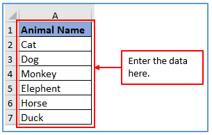
Step 1: Make a Data table first. Here are taken some animal names as information.

Entered the information into the Excel sheet as below.

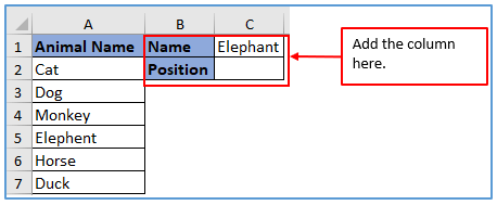
Step 2: Add a column B1:B2 and C1:C2 and write down the animal’s name which you want to get the exact match as a result there.

Added the column here.

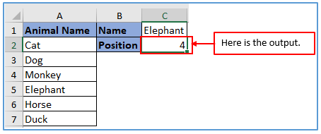
Step 3: Here you can refer to the formula of the exact match of the value and you want to find out the position of elephant. Here C1 is the Exact Match value you wanted to find refer to the ranges A2:A7 and after that refer to 0. Where 0 is MATCH performs an exact match only. The formula is: =MATCH(C2,A2:A7,0)

Applied the formula here.

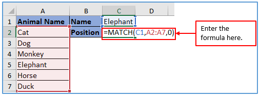
Step 4: Press the enter key and get the Exact value cell number of Elephant where is it.

Here you can see the output is 4 because the elephant is in 4^th position.

3. Types of Match Mode Behavior Information.

Match type is optional. If not provided, the match type defaults to 1 (exact or next smallest). When match type is 1 or -1, it is sometimes referred to as an approximate match. However, keep in mind that MATCH will always perform an exact match when possible, as noted in the table below:

Match type	Behavior	Details
1	Approximate	MATCH finds the largest value less than or equal to the lookup value. The lookup array must be sorted in ascending order.
0	Exact	MATCH finds the first value equal to the lookup value. The lookup array does not need to be sorted.
-1	Approximate	MATCH finds the smallest value greater than or equal to the lookup value. The lookup array must be sorted in descending order.
(omitted)	Approximate	When match type is omitted, it defaults to 1 with behavior as explained above.

4. Apply Multiple criteria in Excel.

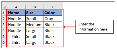
Step 1: First create a dataset like the image below.

Written the information here.

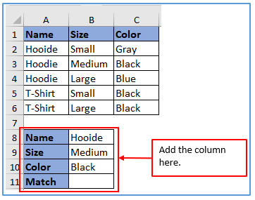
Step 2: Add the column in A8:A11 and B8:B11 B12 to get the multiple criteria result there.

Added the column here.

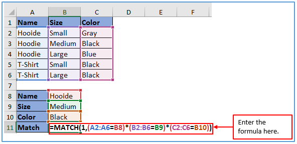
Step 3: Here you can refer to the formula of the match. Here A2:A6 is the range of name value which matches with B8 then you refer * asertic sign for related with each other part. Refer B2:B6 in a range of sizes that match with B10 after that refer C2:C6 so that it matches with B10. The formula will be: =MATCH(1,(A2:A6=B8)*(B2:B6=B9)*(C2:C6=B11))

Applied the formula here.

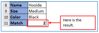
Step 4: Press the enter key and get the Exact value cell number where is it.

Here is the result.

5. Apply Approximate match in Excel.

In the context of spreadsheets and data analysis, an approximate match refers to finding values that are similar to a specified target value, even if they are not identical. This contrasts with an exact match, which requires complete string or numeric equality.

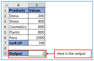
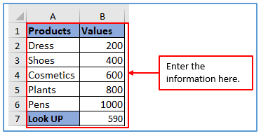
Step 1: You have to make a dataset. Here you can see an example of some products, their values and assuming a look-up value as 590. Placed the information here.

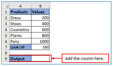
Step 2: Add a column in A9 and B9 to get the result of the approximate match there.

Added the column here as you can see.

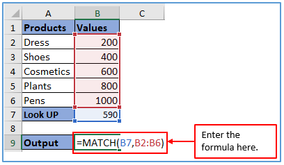
Step 3: Here you can put the match function. Here B7 refers to the lookup value and selects the lookup array B2:B6 after that refer to 1 which shows the approximate value. Use this formula: =MATCH(B7,B2:B6,1)

Used the formula here.

Step 4: Now, click on the enter button and after that you will get the result of it.

The result is outlined below.

Application of Match Function in Excel

Index Matching: Combine MATCH with INDEX to retrieve information from a table based on a lookup value. This provides a flexible alternative to VLOOKUP and HLOOKUP, allowing for leftward searches and dynamic column referencing.
Data Position Identification: Use MATCH to find the position of a specific item within a range or array. This is useful for identifying the rank or order of data elements, such as a product’s sales rank among a list of items.
Dynamic Range References: Employ MATCH within other functions like INDIRECT to create dynamic named ranges. This allows formulas to automatically adjust to data as it expands or contracts, making your formulas more adaptable.
Conditional Formatting: Use MATCH within Conditional Formatting rules to highlight cells that match certain criteria, improving data visualization and making important data stand out.
Data Validation: Incorporate MATCH in data validation rules to restrict data entry to a list of valid options, enhancing data integrity and reducing errors.
Cross-Referencing Data: Utilize MATCH to cross-reference between different data sets, verifying whether items in one list appear in another and identifying mismatches or unique entries.