Lookup and Reference Functions in Excel are indispensable tools for efficient data management and analysis. By mastering these functions, you can streamline the process of searching, retrieving, and cross-referencing data across extensive spreadsheets. Whether you’re compiling reports, analyzing financial records, or managing large datasets, these functions offer the precision and flexibility needed to navigate complex information with ease. Embrace the full potential of Excel’s lookup and reference capabilities to enhance your productivity, reduce errors, and unlock deeper insights from your data.
This Tutorial Covers:
- Excel COLUMN Function
- What it Returns
- Syntax
- Input Arguments
- How to use Column Excel Function (Examples)
- Important notes to remember
- Excel COLUMNS Function
- What it Returns
- Syntax
- Input Arguments
- How to use COLUMNS Excel Function (Examples)
- Important notes to remember
- Excel ROW Function
- What it Returns
- Syntax
- Input Arguments
- How to use ROW Excel Function (Examples)
- Important notes to remember
- Excel ROWS Function
- What it Returns
- Syntax
- Input Arguments
- How to use ROWS Excel Function (Examples)
- Important notes to remember
- Excel HLOOKUP Function
- What it Returns
- Syntax
- Input Arguments
- How to use HLOOKUP Excel Function (Examples)
- Important notes to remember
- Excel VLOOKUP Function
- What it Returns
- Syntax
- Input Arguments
- How to use VLOOKUP Excel Function (Examples)
- Important notes to remember
- Excel XLOOKUP Function
- What it Returns
- Syntax
- Input Arguments
- How to use XLOOKUP Excel Function (Examples)
- Important notes to remember
- Excel INDIRECT Function
- What it Returns
- Syntax
- Input Arguments
- How to use INDIRECT Excel Function (Examples)
- Important notes to remember
- Excel OFFSET Function
- What it Returns
- Syntax
- Input Arguments
- How to use OFFSET Excel Function (Examples
- Important notes to remember:
- Excel FILTER Function
- What it Returns
- Syntax
- Input Arguments
- How to use FILTER Excel Function (Examples)
- Important notes to remember
1. Excel COLUMN Function
To find the target cells’ column numbers in Excel, utilize the column function. Although it is a built-in worksheet function and only requires one argument, the target cell indicates that this function does not return the value of the cell because it only returns the column number. Simply put, the output of this Excel column formula will be a numeric value that represents the specified reference’s column number.
- What it Returns:
It gives back a number that denotes the cell’s selected column’s number. For instance, because B is the second column, =COLUMN(B4) would return 2.
- Syntax:
The following demonstrates the syntax for Excel’s Column Function.
=COLUMN([reference])
- Input Arguments:
[reference]: A cell or group of cells is referenced in this optional argument. The COLUMN function returns the column number of the cell that contains the formula if this parameter is missing.
- How to use Column Excel Function?
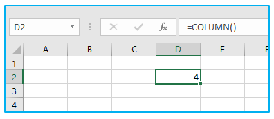
As demonstrated below, if the reference is left out or missing, the column function will provide the column number of the current cells that contain the column formula.
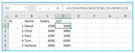
Excel’s column function using the vlookup function:
The column function is compatible with other functions. As an illustration, this function is combined with the lookup function in this place.
Let’s say we have employee data with columns for ID, name, and salary. Additionally, we must deduce the name from the ID. Then, as seen below, we may combine this method with the VLOOKUP function.
- Important notes to remember:
- The COLUMN function returns the column number of the left-most column in the supplied range if the reference is a range of cells. For instance, =COLUMN(B2:D10) would yield 2 because B2 is the leftmost column and 2 is its column number.
- The COLUMN method returns all of the column numbers for the array’s columns if the reference is given as an array.
- Reference cannot make more than one reference or address reference.
- When you need a row of numbers, the COLUMN function can be especially useful. For instance, enter =COLUMN() and drag cell A1 to the right. You will have the numbers 1.2.3 in sequence.
2. Excel COLUMNS Function
Microsoft Excel comes with a built-in feature called COLUMNS. It belongs to Excel’s LOOKUP function category. The COLUMNS function calculates the total number of columns in the array or group of references that is passed as an argument. Knowing the number of columns in an array of references is the goal of Excel’s COLUMNS formula.
- What it Returns:
It gives back a number that indicates how many columns there are overall in the supplied range or array.
- Syntax:
The following demonstrates the syntax for Excel’s COLUMNS Function.
=COLUMNS(array)
- Input Arguments:
array: It could refer to a contiguous group of cells, be an actual array, or be an array formula.
- How to use COLUMNS Excel Function?
Here are two instances of how to operate the COLUMNS function in Excel.
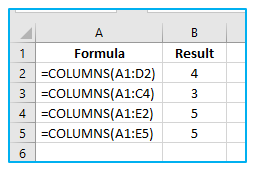
Counting the number of columns in an array:
Because it covers one row, =COLUMNS(A1:D2) returns 4 in the example below (which is A1). Additionally, since the array A1:C4 contains four columns, =COLUMNS(A1:C4) returns 3.
Additionally, keep in mind that it simply counts the number of columns. Therefore, regardless of whether the array is A1:E2 or A1:E5, it would always return 5.
Displaying a sequence of numbers in a Column:
A series of integers can be obtained using the Excel COLUMNS function. Since the first reference is fixed, as you copy the formula down, the row numbers in the array and the second reference both changes.
- Important notes to remember:
- Only the columns are counted, regardless of how many rows and columns the array has.
As an illustration, COLUMNS(A1:B1) returns 2.
Also returned by COLUMNS(A1:B100) is 2.
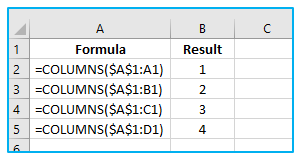
- When you want to acquire a series of numbers as you move to the right in your worksheet, this formula can be helpful.
- Use the formula =COLUMNS($A$1:A1), for instance, if you want 1 in column A1, 2 in column B1, 3 in column C1, and so on. The reference within would change as you dragged it to the right, and the reference’s number of columns would increase by one. Dragging it to column B1, for instance, changes the calculation to COLUMNS($A$1:B1), which then returns 2.
3. Excel ROW Function
The ROW function in Excel displays the current index number of the row of the chosen or target cell. It is a worksheet function in Excel. It is an internal function that only accepts one argument, the reference. The following is how to use this function: =ROW( Value ). ( Value ). Only the cell’s row number and not its value will be displayed.
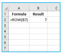
For instance, because A5 is the fifth row in the Excel spreadsheet, the expression =ROW(A5) gives 5.
- What it Returns:
It gives back a number that corresponds to the reference’s row number. As B5 is in the fifth row, for instance, =ROW(B5) would return 5.
- Syntax:
The following demonstrates the syntax for Excel’s ROW Function.
=ROW([reference])
- Input Arguments:
[reference]: A cell or group of cells is referenced in this optional argument. In the absence of this input, the ROW function returns the row number of the cell containing the formula.
- How to use the ROW Excel Function?
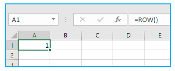
Obtaining the row number of the currently selected cell:
Any cell that has the formula =ROW() entered into it will yield the cell’s row number.
Obtaining the Row Number of a Specified Cell:
The row number of a cell reference is returned if you use the ROW function to supply a cell reference.
- Important notes to remember:
- The row number of the topmost row in the designated range is returned by the ROW function if the reference is a range of cells. For instance, =ROW(B5:D10) would yield 5 because B2 is the top-most row and has a row number of 5.
- The ROW function returns the row numbers for each row in the array if the reference is given as an array.
- Reference cannot make more than one reference or address reference.
- When you need a series of numbers in a column, the ROW function can be especially useful. Put =ROW(), for instance, in cell A1 and drag it downward. You will have the numbers 1.2.3 in sequence.
4. Excel ROWS Function
Simply put, Excel’s “ROWS” function returns the count of the number of rows that are currently chosen in the range. The ROW function, which provides the row number for the selected cell, is different from this. Instead, the ROWS function gives us the number of rows in an array of rows that it is given as an input. Additionally, it serves as a reference function to determine how many rows are there in an array.
- What it Returns:
It gives back a number that indicates how many rows there are overall in the supplied range or array.
- Syntax:
The following demonstrates the syntax for Excel’s ROWS Function.
=ROWS(array)
- Input Arguments:
array: It could refer to a contiguous group of cells, be an actual array, or be an array formula.
- How to use ROWS Excel Function? (Examples)
Knowing how many rows there are in an array:
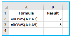
Since only two-row is covered in the below example, =ROWS(A1:A2) yields 2. (which is A2). The array A1:A5 covers five rows in it, therefore =ROWS(A1:A5) yields 5.
Displaying a sequence of numbers in a column:
A series of numbers can be obtained using the Excel ROWS function. Since the first reference is fixed, as you copy the formula down, the row numbers in the array and the second reference both changes.
- Important notes to remember:
- Only the rows are counted, regardless of how many rows and columns are present in the array.
For instance,
ROWS(A1:B3) should output 3.
ROWS(A1:B100) would give 100 results.
- When you want to get a series of numbers as you move along the rows in your worksheet, the ROWS formula can be helpful.
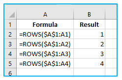
- Use the following formula, for instance, if you want 1 in A1, 2 in A2, 3 in A3, and so on. The reference contained within it would alter as you dragged it downward, increasing the reference’s number of rows by one. Dragging it to row A2, for instance, changes the calculation to ROWS($A$1:A2), which then returns 2.
5. Excel HLOOKUP Function
HLOOKUP, which stands for horizontal lookup, can be used to find data in a table by searching a row for the appropriate information and then printing it from the relevant column. HLOOKUP looks for the value in a row, but VLOOKUP looks for it in a column.
- What it Returns:
It returns the result that matches the criteria.
- Syntax:
The following demonstrates the syntax for Excel’s HLOOKUP Function.
=HLOOKUP(lookup_value, table_array, row_index_num, [range_lookup])
- Input Arguments:
lookup_value: In the first row of the table, this is the look-up value you are seeking. It might be a text string, a cell reference, or a value.
table_array: This is the table in which you are looking for the value. This could be a reference to a named range or a set of cells.
row_index: This is the row number that you wish to retrieve the appropriate value from. The function would return the lookup value if row index was 1. (as it is in the 1st row). The function would return the value from the row immediately below the lookup value if row index was 2, for example.
[range_lookup] (Optional): Here, you can specify whether an exact match or an approximation of a match is desired. It defaults to TRUE – approximate match if missing.
- How to use HLOOKUP Excel Function? (Examples)
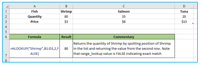
Suppose we have the table of data below.
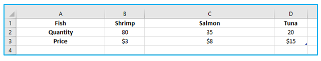
Follow the instructions listed below to utilize the HLOOKUP function:
Step 1: Select the cell where the HLOOKUP formula should be applied by clicking it and typing as below.
=hlookup(
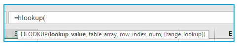
Step 2: In this case, our objective is to fetch Shrimp’s quantity using Horizontal Lookup.
So, we will try to apply an HLOOKUP to get the result.
Type the formula as below.
=HLOOKUP(“Shrimp”,B1:D3,2,FALSE)
‘lookup_value’: As we know that we have to find the quantity of Shrimp, so our ‘lookup_value’ will be a “Shrimp”.
‘table_array’: In this argument, we identify our table by its reference, B1:D3.
‘row_index_num’: The ‘row_index_num’ in this case, would be 2 as here we have to fetch a value from the second row of the table.
‘range_lookup’: Since we only want to retrieve the exact match value in this case, “range_lookup” will return FALSE.
- Important notes to remember:
- Case insensitivity is used while performing a horizontal lookup. This implies that “SHRIMP” and “shrimp” are treated equally.
- The top row of the table_array should always include the “lookup_value” when using the HLOOKUP function.
- The argument “range_lookup” is optional. HLOOKUP uses TRUE as the default value if it is omitted (approximate match).
- When range_lookup is TRUE (approximate match) and HLOOKUP is unable to locate the lookup_value, it uses the greatest value that is less than the lookup_value.
- HLOOKUP issues a #N/A error if “range_lookup” is FALSE and it is unable to locate the lookup_value within the specified range.
- The #VALUE! error is returned by HLOOKUP if the ‘row_index num’ is less than 1. It returns a #REF! error if the value exceeds the number of columns in the table_array.
6. Excel VLOOKUP Function
Vertical Lookup is known as VLOOKUP. It is a function that instructs Excel to look for a specific value in one column (referred to as the “table array”) in order to return a value from another column in the same row.
- What it Returns:
The matching value from a table.
- Syntax:
The following demonstrates the syntax for Excel’s VLOOKUP Function.
=VLOOKUP(lookup_value, table_array, col_index_num, [range_lookup])
- Input Arguments:
lookup_value: This is the look-up value that you are attempting to locate in the table’s left-most column. It might be a value, a reference to a cell, or a text string.
table_array: This is the table array where the value is located. This could be a name for a named range or a pointer to a set of cells.
col_index: This is the column index that you want to retrieve the matching value from
[range_lookup]: You can give an exact match or an approximation here ([range lookup]). It defaults to TRUE – approximate match if left out.
- How to use VLOOKUP Excel Function? (Examples)
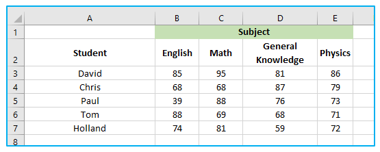
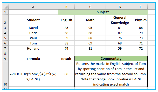
The student names are listed in the left-most column of the VLOOKUP example below, and the grades for the various topics are listed in columns B through E.
Follow the instructions listed below to utilize the VLOOKUP function:
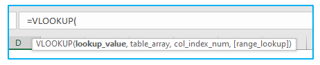
Step 1: Select the cell where the VLOOKUP formula should be applied by clicking it and typing as below.
=vlookup(
Step 2: In this case, our objective is to fetch Tom’s mark in English subject using Vertical Lookup.
So, we will try to apply an VLOOKUP to get the result.
Type the formula as below.
=VLOOKUP(“Tom”,$A$3:$E$7,2,FALSE)
There are four arguments in the formula above:
“Tom”- This is the value for the lookup.
$A$3:$E$7 – This is the range of cells in which we are looking. Remember that Excel looks for the lookup value in the left-most column. In this example, it would look for the name Tom in A3:A7 (which is the left-most column of the specified array).
2 – After identifying Tom’s name, the function will move to the second column of the array and return the value that is located in the same row as Tom. The number 2 in this case signifies that we are seeking for the score from the second column of the given array.
FALSE – It instructs the VLOOKUP function to only check for precise matches.
- Important notes to remember:
- Depending on range_lookup, the match may be precise (FALSE or 0) or approximate (TRUE or 1).
- Make sure the list is ordered from top to bottom before performing an approximate lookup; otherwise, the outcome might not be accurate.
- When data is sorted ascending and range_lookup is TRUE (approximate lookup):
- The greatest value, which is smaller than the lookup_value, is returned if the VLOOKUP method is unable to locate the value.
- If the lookup_value is less than the smallest value, a #N/A error is returned.
- The usage of wildcard characters is possible if lookup_value is text.
7. Excel XLOOKUP Function
Older functions like VLOOKUP, HLOOKUP, and LOOKUP have been replaced by the flexible and up-to-date Excel XLOOKUP function. Wildcards (*?) for partial matches, approximate and exact matching, and lookups in either vertical or horizontal ranges are all supported by XLOOKUP.
- What it Returns:
Matching value(s) from the return array
- Syntax:
The following demonstrates the syntax for Excel’s XLOOKUP Function.
=XLOOKUP(lookup, lookup_array, return_array, [not_found], [match_mode], [search_mode])
- Input Arguments:
- lookup – The value used for lookup.
- lookup array: The array or search range.
- return array: The array or range to be returned.
- not found – [optional] Value to return in the absence of a match.
- match mode – [optional] 0 indicates an exact match (the default), -1 the next smallest exact match, 1 the next largest exact match, and 2 the wildcard match.
- search mode: [optional] Search options include 1 (the default), -1 (from last), 2 (binary ascending), and -2 (binary descending).
- How to use XLOOKUP Excel Function? (Examples)
Procedure of using XLOOKUP Excel Function:
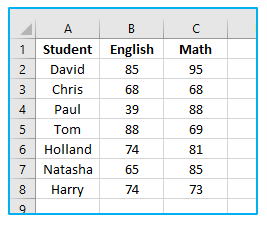
Step 1: Assume you want to retrieve Tom’s English mark from the dataset below (the lookup value).
Select the cell where the XLOOKUP formula should be applied by clicking it and typing the formula as below.
=XLOOKUP(E2,A2:A8,B2:B8)
The result looks like below.
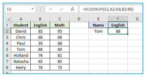
We have only used the necessary inputs in the formula above, which searches for the name (from top to bottom), finds an exact match, and then returns the matching value from B2:B8.
- Important notes to remember:
- XLOOKUP is compatible with both horizontal and vertical arrays.
- If the lookup value cannot be retrieved, XLOOKUP will return #N/A.
- XLOOKUP will return #VALUE if the lookup array’s dimension is incompatible with the return array argument.
- Both workbooks must be open in order to use XLOOKUP between them; otherwise, XLOOKUP will return #REF!.
- Similar to the INDEX function, the output of XLOOKUP is a reference.
8. Excel INDIRECT Function
When you wish to retrieve the values from references to a cell or a range that are text strings, you can utilize Excel’s INDIRECT function.
In summary, you can return the reference indicated by the text string using the indirect formula.
- What it Returns:
A reliable reference for worksheets.
- Syntax:
The following demonstrates the syntax for Excel’s INDIRECT Function.
=INDIRECT(ref_text, [a1])
- Input Arguments:
Ref_text: It is a text string that carries a cell or named range’s reference. The function would return a #REF! error if this wasn’t a legitimate cell reference.
[a1]: A logical value indicating the type of reference to utilize for the text reference. It’s possible for this to be TRUE (signifying an A1 style reference) or FALSE (indicating R1C1-style reference). It is TRUE by default if omitted.
- How to use INDIRECT Excel Function? (Examples)
Procedure of using INDIRECT Excel Function:
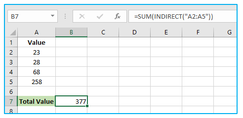
Step 1: Suppose you have a set of values and you want to determine total value of this.
Select the cell where the VLOOKUP formula should be applied by clicking it and typing as below.
=SUM(INDIRECT(
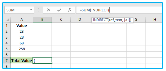
Step 2: Now, you have to refer to the range A2:A5 and give quotation mark. After that, press the enter key on your keyboard.
The result looks like below.
- Important notes to remember:
- The volatile function is INDIRECT. This indicates that it performs a new calculation each time the Excel workbook is opened or a worksheet calculation is initiated. This lengthens the processing time and makes your workbook slower. While the indirect method can be used with small datasets with little to no influence on speed, using it with large datasets may result in your worksheet running more slowly.
This could be the Reference Text (ref text):
- A reference to a cell that itself contains a reference formatted in the A1-style or R1C1-style.
- A cell citation enclosed in double quotations.
- A designated range with a reference return
9. Excel OFFSET Function
The value of a cell or range (of adjacent cells) that is a specific number of rows and columns from the reference point is returned by the OFFSET function in Excel. The initial cell given to the function as a parameter serves as this reference point. The function calculates an end point (finishing cell or range) starting from the reference point and returns its value.
- What it Returns:
It gives back the reference that the OFFSET function is pointing to.
- Syntax:
The following demonstrates the syntax for Excel’s OFFSET Function.
=OFFSET(reference, rows, cols, [height], [width])
- Input Arguments:
reference: The reference you wish to offset from. This could be a reference to a specific cell or a group of nearby cells.
rows: the quantity to be offset in rows. When a positive or negative number is used, the offset is made in the rows below or above, respectively.
cols: It is the number of offset columns. If a positive number is used, the offset is to the right of the columns; if a negative number is used, the offset is to the left of the columns.
[height]: It is an integer that indicates how many rows there are in the returned reference.
[width]: It is a numeric indicator of the returned reference’s column count.
- How to use OFFSET Excel Function? (Examples)
Assume you have the information in the column as follows:
Procedure of using OFFSET Excel Function:
Step 1: Use the following formula in cell E2 to determine the final cell in the column:
=OFFSET(B2,COUNT(B:B)-1,0)
After pressing enter key on your keyboard, the result looks like below.
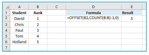
This formula assumes that there are no values other than those displayed and that there are no blank cells in the cells in question. It operates by calculating the amount of filled cells overall and offsetting cell B2 in accordance.
- Important notes to remember:
- No cells are moved by OFFSET; it merely returns a reference.
- Negative values for both rows and cols can be used to reverse the direction of the offsets: negative rows are offset above, while negative cols are offset to the left.
- Because OFFSET is a “volatile function,” it will update every time a worksheet is changed. Volatile functions can slow down the performance of larger and more complicated workbooks.
- If the offset is outside the worksheet’s edge, OFFSET will display the #REF! error value.
- The height and width of the reference are utilized if height or width is missing.
- Any other function that anticipates receiving a reference can utilize OFFSET.
- Although the Excel documentation states that width and height cannot be negative, negative values are valid.
10. Excel FILTER Function:
The Excel FILTER function uses predetermined criteria to filter a set of data. FILTER returns complete rows and all matching entries, unlike most lookup functions. An output dynamic array is the outcome.
- What it Returns:
A changing array of filtered values.
- Syntax:
The following demonstrates the syntax for Excel’s FILTER Function.
=FILTER( array, include, [if_empty] )
- Input Arguments:
array: The filtering range or array
include: A Boolean array for filtering purposes
if_empty (Optional): The message that will appear if none of the entries meet the inclusion criteria
How to use FILTER Excel Function?
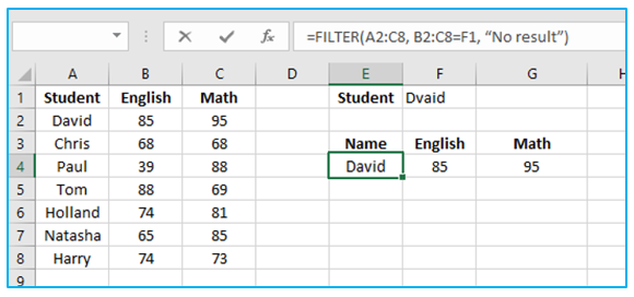
Assume you have the information in the column as follows:
In this example, the range A2:C8 is given as the array to be filtered, and then we set the student column B2:C8 equal to our lookup value in F1 for the include argument to create a Boolean array. As you can see, a result is found when the lookup value is “David” because the basic inclusion condition only displays exact matches.
- Important notes to remember:
- The FILTER function can be used to filter both horizontal and vertical arrays.
- Make sure that both workbooks are open before using the FILTER feature between them. The function will return a #REF! error if they are not.
- If your data is organized this way, the FILTER function will flood the result, therefore make sure there are enough empty cells to the right and below. If you don’t, a #SPILL error will be returned by the function.
- If the dimensions provided in the include parameter are incompatible with the array argument, the FILTER function gives a #VALUE! error.
- Office 365 introduces the FILTER function, which is not present in Office 2019 or prior versions.
