The MOD Function in Excel is a powerful tool for mathematical operations, especially when dealing with division. This function returns the remainder after a number is divided by a divisor. Ideal for various applications, from financial calculations to data analysis, the MOD Function is simple to use yet highly effective in dealing with repetitive division operations. In this guide, we’ll explore the basics of using the MOD Function in Excel, providing step-by-step instructions and practical examples to help you master this essential Excel feature. Whether you’re a beginner or an experienced user, understanding how to effectively utilize the MOD Function can significantly enhance your data handling and analysis capabilities in Excel.
This Content covers:
- What is the modulus Function?
- Apply Basic Calculations using the MOD function.
- How to use the MOD formula to sum every Nth row or column?
- Apply Concatenate Every Nth Column.
- Apply Excel MOD function – syntax.
- How to Use Excel MOD with Data Validation?
1. What is modulus Function?
The modulus function is used to find the remainder when two numbers are divided. Module functions are represented by the symbol “%”. Often used in Excel formulas and calculations to determine what remains after dividing one number by another. The Modulus function is useful in a variety of scenarios, such as when you need to create conditional formatting rules or when you need to calculate periodic patterns in your data. This is a built-in function in MS Excel and is classified as a math/trigonometric function. You can also use this as a worksheet function in Excel. This means that you can enter the MODULUS function in Excel as part of a formula in a worksheet cell.
3 things you about MOD in Excel
- The result of the MOD function has the same sign as the divisor. If the divisor is 0, MOD returns the #DIV/0! error because you cannot divide by zero. If the number MOD is often seen in formulas that deal with “every nth” value.
- MOD is useful for extracting the time from a date. MOD always returns a result in the same sign as the divisor.
- MOD will return a #DIV/0! error if divisor is zero. To discard the remainder and keep the integer, see the QUOTIENT function.
2. Apply Basic Calculations using the MOD function in Excel.
For Basic Calculations using the MOD function, there are written steps below with an example.
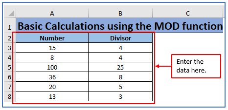
Step 1: Create a data table following with the information below.
Making a table placed with needed information.
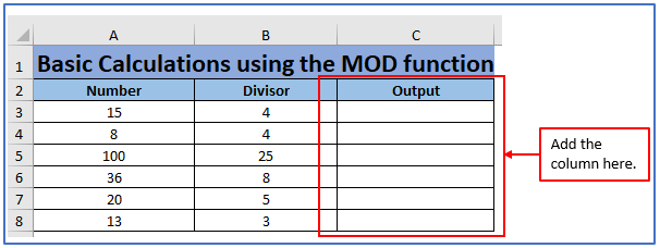
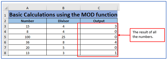
Step 2: Add a column C2:C8 to get the results there and named it Output.
Added a column here.
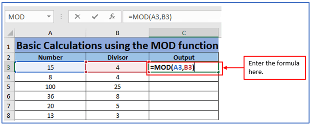
Step 3: Here the formula should be placed according to the data. In the below image you can see that, for the first calculation 15 is in A3 and 4 is in B3. So the formula will be: =MOD(B3,C3).
The formula is used in the image below.
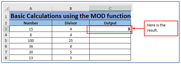
Step 4: Now, press Enter and you will get the result as below.
Here is the result. In the example below, you can see that =MOD(15,4) returns 3 because dividing 15 by 4 gives a remainder of 3.
Step 5: Like the way above, use the same formula with changing column number and you will the result. For number 8 and divisor 4, the formula will be=MOD(B4, C4). You can follow this for the rest of the information.
All the outputs are here. The expression MOD(8,4) returns 0. 8 is divided by 4 with no remainder, and number 100,20 is divided by 25and 5 with no remainder. Also, 36,13 divided by 8,3 with the remainder of 4,1.
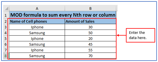
3. How to use the MOD formula to sum every Nth row or column?
Step 1: Here you need to first take some data and make an example.
The below image shows some data about the product name and amount of sales.
Step 2: Add a column to get the results for sales of products there.
Added a column here.
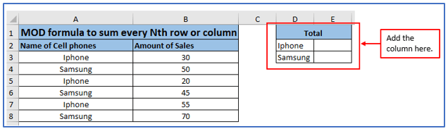
Step 3: Now calculate the Sum of odd row in Column E2.
For this the formula will be:
=SUMPRODUCT((MOD(ROW($C$3:$B$8),2) =1)*($C$3:$C$8))
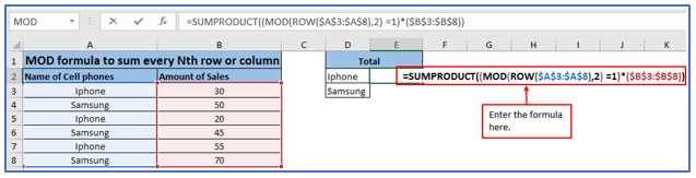
Step 4: Press enter and the result will come out.
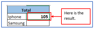
Here is the result below after using the formula for ODD rows:
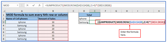
Step 5: For the sum of even rows the formula will be:
=SUMPRODUCT((MOD(ROW( $A$3:$A$8),2)=0)*($B$3:$B$8))
Step 6: Press enter and the result will come out.
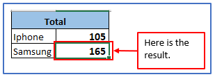
Here is the result below after using the formula for EVEN rows:
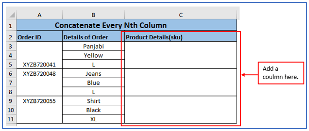
4. Apply Concatenate Every Nth Column.
This feature is especially useful when some details of a product span different cells. When you have a long list of products like this, it becomes a difficult task and that’s where the mod formula comes in.
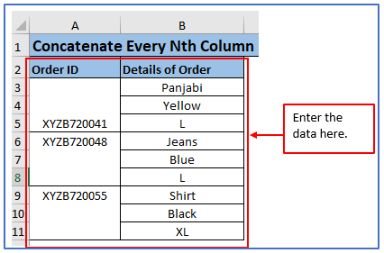
Here is a list of products within a retail business and it needs to sort the data by product details. These details are already visible in column B under ‘Order Details’ and the MOD feature helps you connect these details to create a product ID.
Step 1: First, make some data and put it into excel as shown in the example.
All the data has been placed here.
Step 2: Now, add a column C2:C11 to get the result there and name it Product Details(sku).
Column has added.
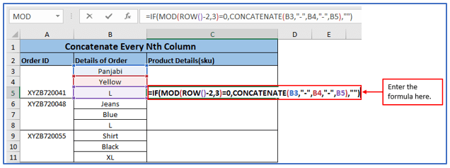
Step 3: Use a MOD expression using the IF function. The formula will be for this example: =IF(MOD(ROW()-2,3)=0,CONCATENATE(B3,”-“,B4,”-“,B5),””)
Applied the formula in the below image.
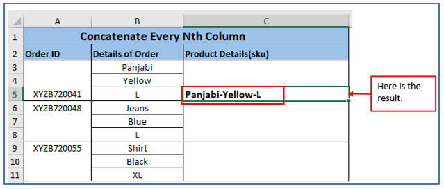
Step 4: After using the formula press Enter.
Here is the result below:
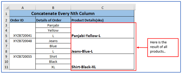
Step 5: Use the same formula for another two orders.
Order ID: XYZB720048 The formula will be :
=IF(MOD(ROW()-2,3)=0,CONCATENATE(B6,”-“, B7,”-“, B8),””)
Order ID: XYZB720048 The formula will be :
=IF(MOD(ROW()-2, 3)=0,CONCATENATE(B9,”-“,B10,”-“,B11),””)
Here is the final output of all the order.
5. Apply Excel MOD function – syntax.
The syntax of the MOD function is:
=MOD(number, divider) where:
number (required) – the number to divide.
Divisor (required) – Number to divide.
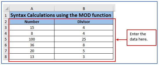
Step 1: Create a data table following with the information below.
Making a table placed with needed information.
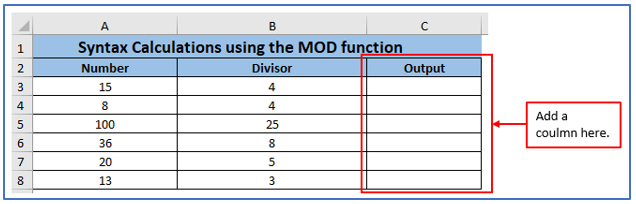
Step 2: Now, add a column C2:C8 to get the output there.
Column has added.
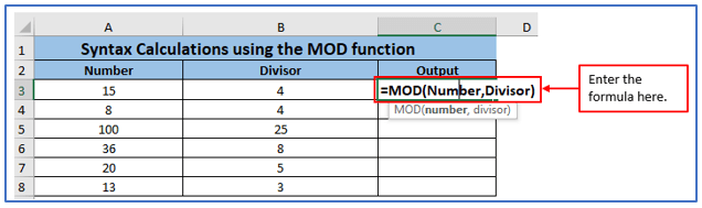
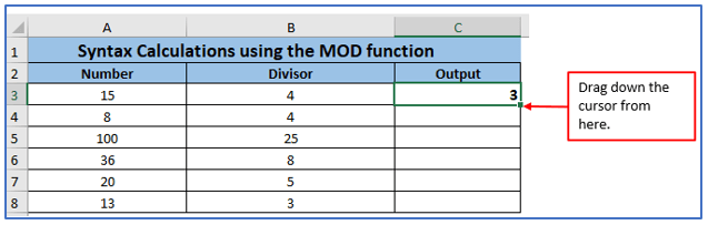
Step 3: Here the formula should be placed according to the data. In the below image, you can see that, for the first calculation 15 is in A3 and 4 is in B3. Enter the formula then click on the number word then click on column A3 which is 15 and then click on Word divisor from formula, click on B3 which is 4.
So the formula will be: =MOD(number,divisor).
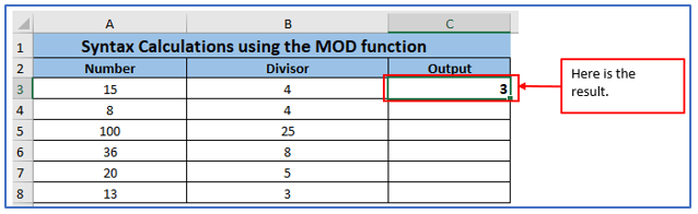
Step 4: Here is the output below.
Step 5: Now, drag down the excel cursor from here or use the same formula from step 3 as shown below.
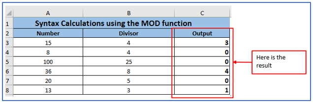
Step 6: The result are outlined.
Here is the result.
6. How to Use Excel MOD with Data Validation?
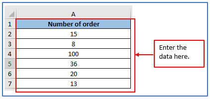
Step 1: Create a data table following with the information below.
Here is the table placed with needed information.
Step 2: Now, select a column to get the output for odd numbers and even numbers there.
Column has added.
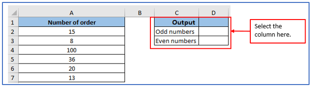
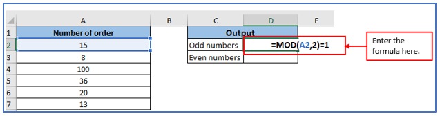
Step 3: Allow only odd numbers the formula will be: =MOD(A2,2)=1, For Even numbers:
=MOD(A2,2)=0
Use this formula according to the column. Choose any column as you want and put the formula.
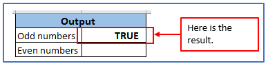
Step 4: Press enter. If the number is odd then it will show the output as true or else False.
Here is the output.
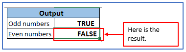
Step 5: Using the even formula for column A7: =MOD(A7,2)=0
and the output is FALSE because 13 is not an even number.
Here is the result.
You may be interested:
