LINEST function in Excel empowers you to delve deep into your data, uncovering valuable insights and predicting trends with precision. Whether you’re analyzing financial data, conducting scientific experiments, or simply making data-driven decisions, LINEST is your trusty companion. Its versatility and accuracy make it an indispensable tool for professionals across various fields. With LINEST in Excel, you have the power to unlock the potential hidden within your data, helping you make informed choices and drive success in your endeavors. Harness the analytical prowess of LINEST function in Excel to elevate your data analysis game and stay ahead in today’s data-driven world.
- What is LINEST Function?
- How to use LINEST function in Excel?
- Apply Excel LINEST function – syntax and basic uses.
- Apply Forecasting with LINEST (Multiple Linear Regression)
- Apply Forecasting with LINEST (Simple Regression)
1. What is the LINEST Function?
The LINEST work in Excel may be a factual work that’s utilized to calculate the least-squares regression line for a set of information. It is regularly utilized in information examination and measurable modeling to discover the best-fit direct condition that represents the relationship between two sets of information focuses. The LINEST work returns an array of values that speak to different measurements of the straight backslide show, counting the standard error, captured, relationship coefficient, and standard mistake, among others.
2. How to use the LINEST function in Excel?
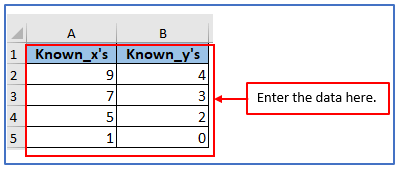
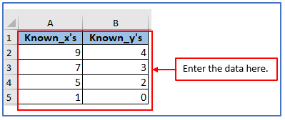
Step 1: Organize the data as shown, and make a table. Here wil Compute line or slope statistics using the LINEST function for the given values. The formula of linest function syntax is: =LINEST(known_y’s, [known_x’s], [const], [stats])
Placed the data into the table.
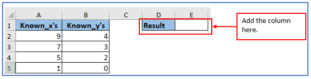
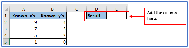
Step 2: Choose a column and name it as result of LINEST function.
The column has been added.
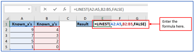
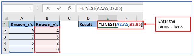
Step 3: Type the formula =LINEST(A2:A5,B2:B5,FALSE).
The above formula shows that A2:A5 is known_xs and B2:B5 is known_ys.
Applied the formula here.
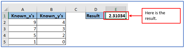
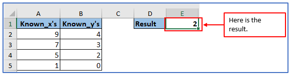
Step 4: Press Enter
The output for the given data will be ‘2.31034’ as shown above.
3. Apply Excel LINEST function – syntax and basic uses.
The LINEST function computes the statistics of a line that describes the relationship between an independent variable and one or more dependent variables and returns an array that describes the line.
This function uses least squares to find the best fit for your data.
where: y – dependent variable to predict.
x- Independent variables used to predict.
a – Intercept (indicates where the line intersects the Y-axis).
b – Slope (indicates the steepness of the regression line, i.e.
the rate of change in y as x changes).
The formula of linest function syntax is: LINEST(known_y’s, [known_x’s], [const], [stats])
Step 1: Organize the data, and make a table with the independent variable in a separate column and the dependent variable in a separate column as shown.
Step 2: Choose a column in D1 and E1 and name it as a result of LINEST function.
The column has been added.
Step 3: Now use the formula. For LINEST syntax the formula will be: =LINEST(known_y’s, known_x’s], [const], [stats]) or =LINEST(A2:A5,B2:B5)
Below here is used the formula.
Step 4: After using the formula you will get the result and the result is shown.
The result is outlined below.
4. Apply Forecasting with LINEST (Multiple Linear Regression)
Multiple linear regression is a statistical analysis method that permits you to survey the relationship between two or more independent variables and a dependent variable.
It is useful for predicting the value of a dependent variable based on the values of two or more independent variables.
Step 1: Organize the data, and make a table with the independent variable in a separate column and the dependent variable in a separate column.
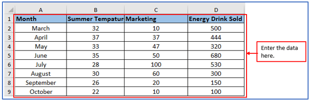
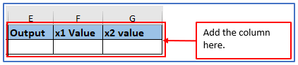
Step 2: Choose the column in E1:E2,F1:F2 and G1:G2 as instructed below.
The column has been added.
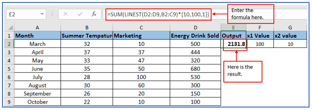
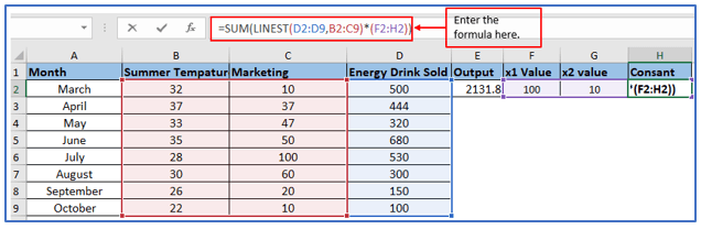
Step 3: Use Equation 10 to calculate the quantity of Energy Drinks sold for promotional purposes. Equation B2:C9 is a set of two independent values (x) and D2:D9.
Variable (y): To calculate sales, you need to multiply the respective coefficients by the x values entered in the array format of the formula {10, 100, 1}. The expression “1” indicates the last value by which the x value is multiplied, the intercept value. Multiple Regression returns the right-to-left slope coefficient.
The formula used is: =SUM(LINEST(D2:D9,B2:C9)*{10,100,1}) and press enter the result is shown below.
Here The ad cost is returned first, and the temperature is returned as the second factor.
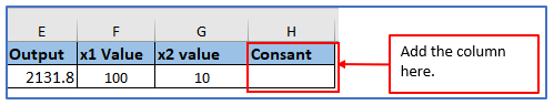
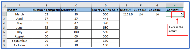
Step 3: Now, Add another column in H1 and H2 name it Consant as instructed below.
The column has been added.
Step 4: Cell references are used instead of entering values directly into cells.
The formula changes to: =SUM(LINEST(D2:D9,B2:C9)*(F2:H2))
Applied the formula here.
Step 5: Press enter and the result will come out.
Here is the result.
5. Apply Forecasting with LINEST (Simple Regression)
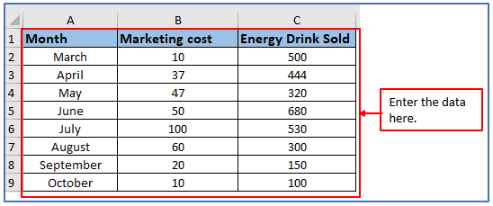
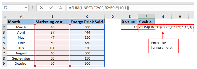
Step 1: Organize the data as shown, and make a table with the independent variable in a separate column B2:B9 and the dependent variable in a separate column C2:C9.
Placed the information here.
Step 2: Now, Add another column in E1,E2 and F1,F2 as instructed below, here X value is marketing cost and you need to find out Y value.
The column has been added.
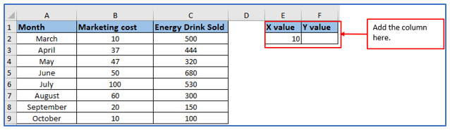
Step 3: In the worksheet, enter the marketing cost for October. Select Cell F2 and use the formula: =SUM(LINEST(C2:C9,B2:B9)*{10,1})
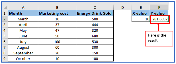
Step 4: By pressing Enter, the y value for an x value will be displayed. Advertising will cost 10 for the number of products being sold.’
You can see below the result. Here is the result. The total sales of the product for October is 281.6697.
Application of LINEST function in Excel
- Linear Regression Analysis: LINEST is commonly used to perform linear regression analysis. It calculates the best-fit straight line through a set of data points, allowing you to understand the relationship between variables.
- Trendline Creation: You can use LINEST to generate trendlines in charts, helping you visualize trends and make predictions based on historical data.
- Forecasting: LINEST can be employed to forecast future values based on the linear relationship established by historical data. This is particularly useful in financial and sales forecasting.
- Quality Control: In manufacturing and quality control, LINEST can help assess the relationship between variables to maintain product quality and identify factors affecting it.
- Scientific Research: LINEST is used in scientific research to analyze experimental data and determine the degree of correlation or causation between variables.
- Financial Analysis: In finance, LINEST can be applied to analyze the relationship between financial variables like stock prices and economic indicators, aiding in investment decision-making.
LINEST is a versatile tool for data analysis, offering insights into various fields by quantifying relationships and making predictions based on historical data.
For ready-to-use Dashboard Templates:
