How to use HLOOKUP Function in Excel?

The three lookup functions in Microsoft Excel, LOOKUP, VLOOKUP, and HLOOKUP, are undoubtedly the ones that cause users the most confusion. In this tutorial, we’ll concentrate on the details of the Excel HLOOKUP function and go over some formula examples to show you how to use it in Excel as effectively as possible.

This Tutorial Covers:

When to Use the Excel HLOOKUP Function
What it Returns
Syntax
Input Arguments
3 points to understand about the Excel HLOOKUP function
Using HLOOKUP Formula in Excel formula examples
- Horizontal lookup with both an approximate and exact match
  - HLOOKUP using an approximate match
  - HLOOKUP using exact match
- How to perform the HLOOKUP formula from a different workbook or spreadsheet
- HLOOKUP in Excel with partial match (wildcard characters)
Excel HLOOKUP’s stronger replacement is INDEX/MATCH
How to use Excel’s case-sensitive HLOOKUP function
Top 10 causes of Excel HLOOKUP malfunction

1. When to Use the Excel HLOOKUP Function?

The Excel HLOOKUP function works best when you are searching for a matching data point in a row and, after finding it, you need to fetch a value from a cell in a column that is a defined number of rows below the top row.

2. What it Returns?

The specified matching value is returned.

3. Syntax:

The following is the syntax:

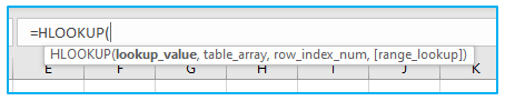
=HLOOKUP(lookup_value, table_array, row_index_num, [range_lookup])

4. Input Arguments:

lookup_value – This is the look-up value you’re searching for in the table’s first row. It might be a text string, a cell reference, or a number.

table_array – this is the table for which you are looking for the value. This could be a reference to a named group of cells.

row_index – This is the row number you need to retrieve the matching data from. The function would yield the lookup value if row_index was 1. (as it is in the 1st row). The function would return the number from the row immediately below the lookup value if row_index was 2, for example.

[range_lookup] – (Optional) Here, you can indicate whether an exact match or an approximation of a match is desired. It sets to TRUE – approximate match if left out. (see additional notes below).

5. 3 points to understand about the Excel HLOOKUP function:

Please keep the following information in mind whenever you perform a horizontal lookup in Excel:

The top row of table_array is the only row that the HLOOKUP function can scan. If you need to seek something up elsewhere, you might want to use an Index/Match formula.
Excel’s HLOOKUP does not differentiate between capital and lowercase letters; it is case-insensitive.
The values of in the first row of table_array must be sorted in ascending order (A-Z), left to right, if range_lookup is set to TRUE or omitted (approximate match).

6. Using HLOOKUP Formula in Excel-formula examples:

As you can see, the Excel HLOOKUP formula is beginning to appear somewhat familiar, let’s explore some additional formula examples to reinforce your understanding of the HLOOKUP function.

Horizontal lookup with both an approximate and exact match:

As you are already aware, based on the value given to the range_lookup argument, Excel’s HLOOKUP function can carry out a lookup with an exact match or a non-exact match:

TRUE or omitted – approximate match

FALSE – exact match

Please remember that even though we state, “approximate match,” any HLOOKUP formula initially looks for an exact match. However, if an exact match cannot be determined, the formula will return an approximate match (the value that is closest to being less than the lookup value); if TRUE or omitted, the formula will instead return the #N/A error.

Consider the following HLOOKUP examples to illustrate the concept more clearly.

HLOOKUP using an approximate match:

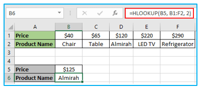
Supposing you have a list of product name in row 2 (B2:F2) and their prices in row 1(B1:F1). You want to find out which product has a certain picture that is input in cell B5.

You cannot rely on the off chance that your staffs know the lookup price exactly, so it makes sense to return a nearest match if an exact value in not found.

For instance, to find out the product whose price is around 125$, use the following formula (range_lookup set to TRUE or omitted as in this example):

=HLOOKUP(B5, B1:F2, 2)

Please remember that an approximate match requires sorting the values in the top row from smallest to largest or from A to Z, otherwise your HLOOKUP formula may return a wrong result.

As you can see in the screenshot below, our formula returns Almirah whose price is 120$

HLOOKUP using exact match:

The final HLOOKUP parameter can be set to FALSE if you are certain of the lookup value.

=HLOOKUP(B5, B1:F2, 2,FALSE)

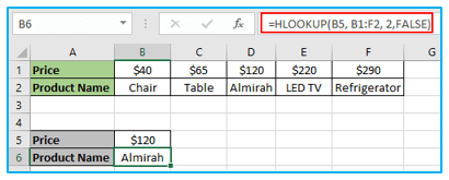
An advantage of using an approximate match Hlookup is that it is more convenient for users as it doesn’t require them to sort data in the first row. However, it’s important to note that if the lookup value is not found exactly, the function will return an #N/A error.

Tip: To avoid frightening your users with N/A errors, you can embed your Hlookup formula in IFERROR and show your own message, for instance:

=IFERROR(HLOOKUP(B4, B1:I2, 2, FALSE), “Sorry, not found”)

How to perform HLOOKUP formula from a different workbook or spreadsheet?

H-lookup from a separate sheet or workbook essentially just means adding external references to your HLOOKUP formula.

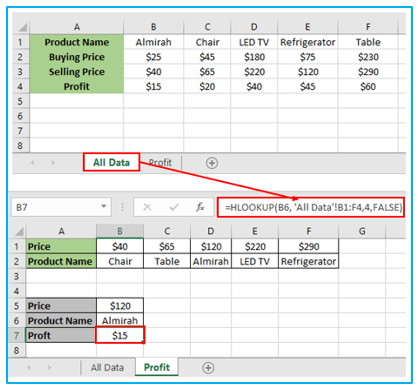
You must give the name of the worksheet followed by an exclamation point if you want to retrieve matching data from a different worksheet. For instance:

=HLOOKUP(B6, ‘All Data’!B1:F4,4,FALSE)

A single quotation mark is not required if the worksheet name does not contain spaces or other non-alphabetical symbols, such as in the following example:

=HLOOKUP(B6, Data!B1:F4,4,FALSE)

Include the name of the referenced workbook in square parentheses whenever it is used:

=HLOOKUP(B6, [Book1.xlsx]Data!B1:F4,4,FALSE)

The full path must be specified if you are extracting data from a closed workbook:

=HLOOKUP(B6, ‘E:\Reports\[Book1.xlsx]All Data’!B1:F4,4,FALSE)

Tip: If you select cells on a different sheet, Excel will instantly add an external reference to your formula rather than requiring you to physically type the names of the workbook and worksheet.

HLOOKUP in Excel with partial match (wildcard characters):

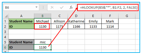
For example, you have a list of student names in row 1 and their IDs in row 2. You want to find the student ID for a specific student but you cannot remember the name exactly, though you do remember it begins with “mic”.

Assuming your data are in cells B1:F2 (table_array) and IDs are in row 2 (row_index_num), the formula goes as follows:

=HLOOKUP(“mic*”, B1:F2, 2, FALSE)

To make the formula more flexible, you can type the lookup value in a special cell, say B5, and concatenate that cell with the wildcard character, like this:

=HLOOKUP(B5&”*”, B1:F2, 2, FALSE)

Notes:

The range_lookup argument must be changed to FALSE for an HLOOKUP formula that uses wildcards to function properly.
The first value discovered is returned if the wildcard conditions are met by more than one value in table_array.

7. Excel HLOOKUP’s stronger replacement is INDEX/MATCH:

As you are already aware, Excel’s HLOOKUP function has a number of restrictions, the two most important of which are that it can only look up values in the top row and that values must be sorted when using an estimated match.

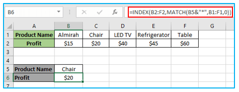
Luckily, there exists a more powerful and versatile option to Vlookup and Hlookup in Excel – the liaison of INDEX and MATCH functions, which boils down to this generic formula:

INDEX (where to return a value from, MATCH (lookup value, where to search, 0))

Assuming your lookup value is in cell B5, you are looking for a match in row 1 (B1:F1), and want to return a value from row 2 (B2:F2), the formula is as follows:

=INDEX(B2:F2,MATCH(B5&”*”,B1:F1,0))

8. How to use Excel’s case sensitive HLOOKUP function?

As was stated at the outset of this tutorial, the Excel HLOOKUP tool does not take case into account. You can use the EXACT function, which compares cells precisely, inside the INDEX MATCH formula discussed in the preceding example when the character case matters:

INDEX (row to return a value from, MATCH(TRUE, EXACT(row to search in, lookup value), 0))

Assuming your lookup value is in cell B5, the lookup range is B2:G2, and the return range is B1:G1, the formula takes the following shape:

=INDEX(B1:G1, MATCH(TRUE, EXACT(B2:G2,B5),0))

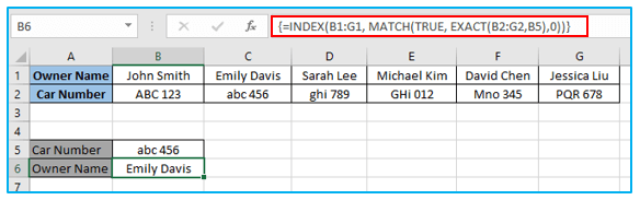
Remember this: You need to enter the formula by pressing Ctrl + Shift + Enter because it is an array formula.

9. Top 10 causes of Excel HLOOKUP malfunction:

The HLOOKUP function in Excel is a powerful and useful tool for performing horizontal lookups in a table. However, it can also be quite tricky to use, and errors such as #N/A, #VALUE, and #REF are not uncommon. If you find that your HLOOKUP formula is not working as expected and if you are wondering why HLOOKUP does not work, it is likely due to one of the following reasons:

The top row of a table is the only row that HLOOKUP can examine. An N/A error will be returned if your lookup numbers are in a different row. Use an INDEX MATCH algorithm to get around this restriction.
When performing a lookup, it is important to determine whether an exact match or an approximate match is required. When searching with an approximate match (range_lookup set to TRUE or omitted), it is essential to sort values in the first row in ascending order.
When using multiple HLOOKUP formulas to retrieve information about a row of lookup values, it is necessary to lock the table array reference to ensure that it remains consistent when copying the formula.
Inserting or deleting a row from a table can cause an HLOOKUP formula to break, as it relies on the row index number you specify. To avoid this issue, either lock the table to prevent users from inserting new rows or use an INDEX MATCH formula instead.
If there are duplicates in the table, HLOOKUP can only return the first matching value. To handle duplicate records, you can remove them using Excel’s built-in tools, use a PivotTable to group and filter your data, or use an array formula to extract all duplicate values.
Extra spaces in the table or lookup value can cause an HLOOKUP formula to return #N/A errors. You can remove these spaces using Excel’s TRIM function.
Text strings that resemble numbers can also cause errors in HLOOKUP formulas.
HLOOKUP can only handle lookup values up to 255 characters in length. If your lookup value exceeds this limit, you will receive a #VALUE! error. To avoid this issue, use an INDEX MATCH formula instead.
When performing an HLOOKUP from another workbook, it is essential to specify the full path to the lookup workbook.
Common errors caused by supplying incorrect arguments include returning a #VALUE! error if row_index_num is less than 1, a #REF! error if row_index_num is greater than the number of rows in table_array, and an #N/A error if you search with an approximate match and your lookup_value is smaller than the smallest value in the first row of table_array.

By being aware of these potential issues and taking steps to avoid them, you can make more effective use of the HLOOKUP function in Excel. However, it is also important to note that alternatives such as INDEX MATCH may be more reliable and flexible in certain situations.

So that’s how you use HLOOKUP in Excel. We hope that this tutorial will be useful to you.

For ready-to-use Dashboard Templates:

How to use HLOOKUP Function in Excel?

Leave a Comment Cancel Reply

Categories