Excel REPLACE and SUBSTITUTE Functions are essential tools for anyone looking to refine and manipulate text data within their spreadsheets. These functions offer unparalleled flexibility in editing and formatting text strings, enabling you to correct errors, update information, and clean imported data with ease. Whether you’re aiming to improve data accuracy, consistency, or readability, mastering these functions will significantly enhance your ability to manage and present data effectively. Embrace the power of REPLACE and SUBSTITUTE to take your Excel data manipulation skills to the next level.
This Tutorial Covers:
- Excel REPLACE function
- Using Excel REPLACE function with numeric values
- Using Excel REPLACE function with dates
- To perform numerous replacements in a cell, use nested REPLACE functions
- replacing a string that appears in a unique location in each cell
- Excel SUBSTITUTE function
- Use a single formula to replace several values (nested SUBSTITUTE)
- Excel REPLACE vs. Excel SUBSTITUTE
1. Excel REPLACE function
You can replace one or more characters in a text string with another character or group of characters using Excel REPLACE function.
=REPLACE(old_text, start_num, num_chars, new_text)
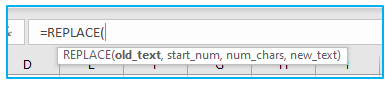
As you can see, the Excel REPLACE function requires all 4 of its inputs.
old_text – The original text (or a pointer to a cell holding the original content) that needs some characters replaced.
start_num – Where the first character in the old text that you wish to replace is located.
num_chars – How many characters you wish to change.
new_text – The replacement text.
Note: One thing to keep in mind is that an Excel Replace formula will return the #VALUE! error if the start num or num chars input is negative or not a number.
- Using Excel REPLACE function with numeric values:
Replace with Excel REPLACE function is made to function with text strings. Of course, you can use it to change any numerical characters in a text string, like:
=REPLACE(A2, 9, 2, “11”)
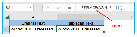
As is customary for text values, “11” is enclosed in double quotes.
You can change one or more digits in a number in a similar way. For instance:
=REPLACE(A2, 4, 4,”3″)
Again, the new value must be enclosed in double quotations (“3”).
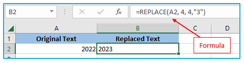
Note: Excel’s REPLACE formula never returns a number; it always produces a text string. Compare the left alignment of the returned text value in B2 in the screenshot above to the original number’s right alignment in A2. Additionally, since it is a text value, you cannot use it in any other calculations without first converting it back to a number.
- Using Excel REPLACE function with dates:
The REPLACE Excel function, as you’ve just seen, works perfectly fine with numbers, but it only produces a text string. You might try using various Replace formulae on dates while keeping in mind that dates are stored as numbers in the internal Excel system. The outcome would be embarrassing.
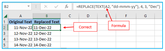
For instance, suppose you want to convert “Nov” to “Dec” in the date in A2, which is 11-Nov-22. In order to instruct Excel to replace 3 characters in cells A2 starting with the 4th character, you enter the formula “=REPLACE(A2, 4, 3, “Dec”)”. and obtained the following outcome:
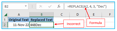
How come that? Because the date “11-Nov-22” is actually only a visual representation of the serial number (44876) underneath. The result of our Replace formula is the text string “448Dec,” which transforms the final three digits of the serial number in the example above to “Dec.”
You can use the TEXT function or any other method described in How to convert date to text in Excel to convert dates to text strings before using the Excel REPLACE function to ensure that dates are handled correctly. As an alternative, you can include the TEXT function right in the REPLACE function’s old_text argument:
=REPLACE(TEXT(A2, “dd-mmm-yy”), 4, 3, “Dec”)
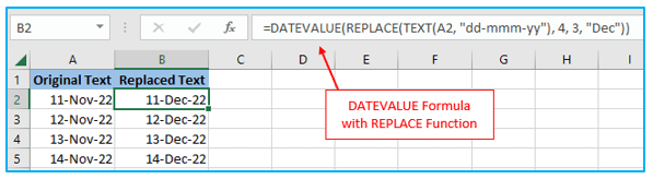
Please keep in mind that the formula’s output is a text string, so this technique only works if you don’t intend to utilize the updated dates in further calculations. Use the DATEVALUE function to convert the values supplied by the Excel REPLACE function back to dates if you actually require dates rather than text strings:
=DATEVALUE(REPLACE(TEXT(A2, “dd-mmm-yy”), 4, 3, “Dec”))
- To perform numerous replacements in a cell, use nested REPLACE functions:
You could frequently need to perform many replacements in a single cell. Naturally, you could perform one replacement, output an interim result into a second column, and then perform the second replacement. However, using nested REPLACE functions, which enable you to carry out several replacements with a single formula, is a better and more professional approach. Nesting in this sense refers to putting one function inside another.
Consider the case below. Let’s say you want to add hyphens to a list of phone numbers structured like “987654321” in column A in order to make them appear more like phone numbers. To translate “987654321” into “987-654-321” is your aim.
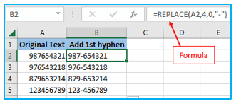
The initial hyphen is simple to insert. You enter the following Excel Replace formula, which inserts a hyphen in the fourth position in a cell to replace the letter zero:
=REPLACE(A2,4,0,”-“)
The following is the output of the Replace formula mentioned above:
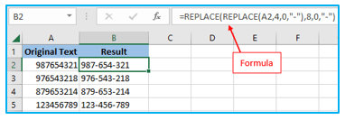
Okay, the eighth slot now requires the addition of one more hyphen. You accomplish this by enclosing the calculation above with another Excel REPLACE function. In order for the second REPLACE function to handle the value returned by the first REPLACE and not the value in cell A2, you must encapsulate it in the old_text argument of the other function.
=REPLACE(REPLACE(A2,4,0,”-“),8,0,”-“)
As a consequence, you receive the phone numbers with the formatting you want:
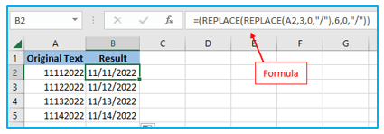
Similar to this, you can make text strings resemble dates by using nested REPLACE functions and inserting a forward slash (/) when necessary:
=(REPLACE(REPLACE(A2,3,0,”/”),6,0,”/”))
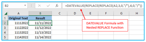
Additionally, you can transform text strings into actual dates by adding the DATEVALUE function to the REPLACE formula mentioned above:
=DATEVALUE(REPLACE(REPLACE(A2,3,0,”/”),6,0,”/”))
Additionally, there is no restriction on how many functions you can nest inside of a single formula (the modern versions of Excel 2010, 2013, 2016, 2019, and 2021 allow up to 8192 characters and up to 64 nested functions in a formula).
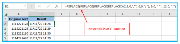
For instance, you may make a number in A2 look like the date and time by using three nested REPLACE functions:
=REPLACE(REPLACE(REPLACE(REPLACE(A2,3,0,”/”),6,0,”/”), 9,0, ” “), 12,0, “:”)
- Replacing a string that appears in a unique location in each cell:
So far, we have replaced values in the identical positions in each cell of all the samples using values of a similar nature. But in reality, projects are frequently more difficult than that. You will need to identify the location of the first character that has to be replaced because it’s possible that the replacement characters won’t always appear in the same spot in each cell in your worksheets. The example that follows will illustrate what I’m getting at.
Imagine you have a column A list of email addresses. And one company’s name has changed from “XYZ” to, let’s say, “YXZ.” Therefore, you must alter every client’s email address to reflect this.
However, the length of the client names poses an issue, making it impossible to identify precisely where the corporate name starts. In other words, you are unsure of the value to enter in the Excel REPLACE function’s start_num argument. Find the first character in the string “@xyz” using the Excel FIND function to find out:
=FIND(“@xyz”,A2)
Afterward, include the aforementioned FIND function in your REPLACE formula’s start_num argument:
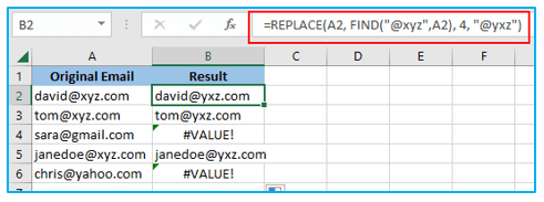
=REPLACE(A2, FIND(“@xyz”,A2), 4, “@yxz”)
Suggestion: To prevent unintentional replacements in the name portion of email addresses, we include “@” in our Excel Find and Replace function. Even if there is a very small probability that these matches may happen, it never hurts to be cautious.
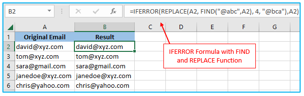
The formula has no trouble locating the old text and replacing it with the new content, as you can see in the screenshot that follows. However, the formula returns the #VALUE! error if the text string that has to be substituted cannot be found.
And rather than returning the error, we want the formula to return the original email address. So, let’s include the IFERROR function in our FIND & REPLACE formula:
=IFERROR(REPLACE(A2, FIND(“@xyz”,A2), 4, “@yxz”),A2)
And it’s true that this enhanced formula functions flawlessly.
The REPLACE function can also be used to capitalize the first letter of a cell’s name. Use the method in the above-linked sentence whenever you are dealing with a list of names, products, or other items to turn the initial letter to uppercase.
Tip: Using the Excel FIND and REPLACE dialog would be an easier approach to perform the replacements in the original data.
2. Excel SUBSTITUTE function
Excel’s SUBSTITUTE function substitutes a particular character for one or more instances of a supplied character or text string (s).
The Excel SUBSTITUTE function has the following syntax:
=SUBSTITUTE(text, old_text, new_text, [instance_num])
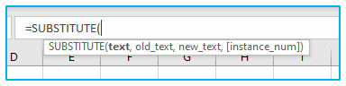
The final argument is optional, but the previous three are necessary.
text – The original text where the characters you want to replace are located. can be provided as a cell reference, a test string, or the outcome of another formula.
old_text – The character or characters you wish to swap out.
new_text – New character(s) to use in place of old text.
instance_num – The instance of old_text that needs to be replaced. If left out, the new text will be substituted for the old text anywhere it appears.
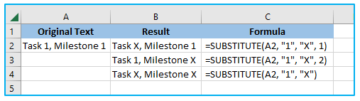
For instance, the following formulas all replace “1” with “X” in cell A2, but they produce various outcomes based on the value you enter in the final argument:
=SUBSTITUTE(A2, “1”, “X”, 1) – Substitutes the first occurrence of “1” with “X”.
=SUBSTITUTE(A2, “1”, “X”, 2) – Substitutes the second occurrence of “1” with “X”.
=SUBSTITUTE(A2, “1”, “X”) – Substitutes all occurrences of “1” with “X”.
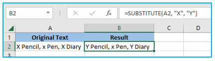
Note: Please take note that Excel’s SUBSTITUTE function is case-sensitive. For instance, the formula that follows changes all instances of the uppercase “X” in cell A2 to “Y,” but it leaves all instances of the lowercase “x” alone.
- Use a single formula to replace several values (nested SUBSTITUTE):
Similar to how the Excel REPLACE function works, you can layer multiple SUBSTITUTE functions inside of a single formula to do multiple replacements simultaneously, or to replace many characters or substrings using a single formula.
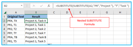
Let’s say cell A2 contains a text string like “PRX, TX,” where “PR” stands for “Project” and “T” represents for “Task.” The two codes should be swapped out for their entire names. You can use two distinct SUBSTITUTE formulae to accomplish this:
=SUBSTITUTE(A2,”PR”, “Project “)
=SUBSTITUTE(A2, “T”, “Task “)
Then nest them within one another:
=SUBSTITUTE(SUBSTITUTE(A2,”PR”,”Project “), “T”,”Task “)
For easier reading, a space has been inserted at the end of each new text argument.
3. Excel REPLACE vs. Excel SUBSTITUTE
Both the Excel REPLACE and SUBSTITUTE functions are made to swap text strings, which makes them quite similar to one another. The following are the distinctions between the two functions:
- SUBSTITUTE changes one or more occurrences of a certain character or text string in a text string. Use Excel’s SUBSTITUTE tool if you are aware of the text that needs to be changed.
- REPLACE modifies characters in a text string at a particular location. Use Excel’s REPLACE function if you know where the character or characters to be replaced are located.
- When using Excel’s SUBSTITUTE function, you can specify which instance of the old_text should be replaced with the new_text by providing the instance_num optional argument.
The SUBSTITUTE and REPLACE capabilities in Excel are utilized in this manner. Hopefully, these examples can help you with your tasks.
Application of Excel REPLACE and SUBSTITUTE Functions
- Correcting Typographical Errors: Use REPLACE to correct common spelling mistakes within a text string by specifying the position of the character to be replaced, enhancing data accuracy.
- Formatting Text Strings: Apply SUBSTITUTE to change formatting within text, such as replacing dashes (-) with slashes (/) in date formats, ensuring consistency across your data.
- Dynamic Template Filling: Utilize SUBSTITUTE to dynamically replace placeholders in a text template with actual data, streamlining the creation of personalized emails or reports.
- Cleaning Data: Employ REPLACE to remove unwanted characters or spaces from data imported from other sources, making it cleaner and more usable for analysis.
- Batch Updating Information: Use SUBSTITUTE to update parts of a string across a dataset, such as changing a product code prefix or company name, maintaining data relevance.
- Creating User-friendly Displays: Apply REPLACE or SUBSTITUTE to modify text data into a more readable format, such as abbreviating or expanding terms, improving data presentation.
For ready-to-use Dashboard Templates:
