How to use Excel INDIRECT Function and Excel OFFSET Function?

Excel INDIRECT Function and Excel OFFSET Function are indispensable tools for advanced data management and analysis, offering unparalleled flexibility and control over your spreadsheets. By mastering these functions, you can dynamically reference data, create adaptable formulas, and manage large datasets with ease. Whether you’re building complex reports, analyzing trends, or managing evolving data sets, the INDIRECT and OFFSET functions empower you to handle data more efficiently and accurately. Integrate these powerful functions into your Excel toolkit to transform your approach to data analysis and make your spreadsheets more responsive and adaptable to change.

This Tutorial Covers:

1. Excel INDIRECT function – syntax and arguments
   • Examples of formulas for using INDIRECT in Excel
     • Creating indirect references from cell values
     • Building indirect references from text and cell values
     • Using the INDIRECT function with named ranges
     • INDIRECT formula that dynamically references a different worksheet
     • Using INDIRECT with other Excel functions
       • Example 1- INDIRECT and ROW functions
       • Example 2- Combination of INDIRECT, ADDRESS, COLUMN and ROW functions

2. Excel OFFSET function – syntax and arguments
   • How to use OFFSET function in Excel – formula examples
     • Excel OFFSET and SUM functions
       • Example 1- A SUM/OFFSET formula that is dynamic
       • Example 2- To sum the last N rows in Excel, use the OFFSET formula
     • Using OFFSET function with AVERAGE, MAX, MIN
     • Making a dynamic range with Excel’s OFFSET formula
   • Excel OFFSET & VLOOKUP
     • Example 1-Vlookup left in Excel using the OFFSET formula
     • Example 2- Two-way lookup (by column and row values)
   • Limitation of OFFSET Function
   • Alternatives to using OFFSET in Excel

1. Excel INDIRECT function – syntax and arguments

Excel INDIRECT is used to indirectly reference cells, ranges, other sheets, or workbooks, as its name implies. In other words, rather than hard-coding cell or range references, you can build them dynamically using the INDIRECT function. This allows you to alter a reference within a formula without altering the formula itself. Furthermore, even if you add or remove existing rows or columns from the worksheet, these indirect references won’t alter.

INDIRECT function syntax:

From a text string, Excel INDIRECT function returns a cell reference. It has two arguments, the first of which is necessary and the second of which is not:

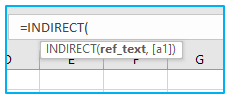
=INDIRECT(ref_text, [a1])

ref_text – is a named range, a cell reference, or a reference to a cell in the form of a text string.

a1 – is a logical value that indicates the kind of reference the ref text parameter contains:

• ref text is treated as an A1-style cell reference if TRUE or omitted.
• ref text is considered as an R1C1 reference if FALSE.

While the R1C1 reference type may be advantageous occasionally, you should usually stick to the well-known A1 references the majority of the time. In any case, A1 references will be used in almost all INDIRECT formulas in this lesson, therefore we will skip the second argument.

• Examples of formulas for using INDIRECT in Excel

When dealing with actual data, the INDIRECT function Excel has the ability to convert any text string into a reference, even incredibly complicated strings that you construct by combining the values of numerous cells and the output of other Excel calculations. To avoid putting the cart before the horse, let’s examine each Excel Indirect formula individually.

I hope all that theory didn’t make you bored. Anyway, the most interesting part is now here, the actual applications of the INDIRECT function.

• Creating indirect references from cell values

The A1 and R1C1 reference styles are supported by the Excel INDIRECT function, as you may recall. Normally, you can only choose between the two reference types via the File > Options > Formulas > R1C1 check box, making it impossible to utilize both styles simultaneously on a single sheet. This is the reason R1C1 is rarely used as an alternate referencing method by Excel users.

Either reference type may be used in an INDIRECT formula on the same sheet if desired. You might want to be aware of the distinction between A1 and R1C1 reference styles before continuing.

The most common reference type in Excel that relates to a column and a row number is A1 style. For instance, the cell at the junction of row 2 and column B is designated as B2.

The R1C1 reference type is the contrary, with rows coming before columns, and it does take some getting used to. For instance, the cell A4 on a sheet’s row 4, column 1, is referred to as R4C1. When a letter is followed by a number, you are referring to the same row or column.

Let’s now examine how the INDIRECT function manages references to A1 and R1C1:

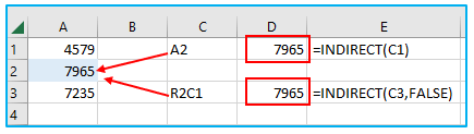
The output of three distinct Indirect formulas is the same, as shown in the screenshot above.

In cell D1 is the following formula: =INDIRECT(C1)

The simplest one is this one. The formula makes a reference to cell C1, retrieves its value, which is the text string A2, turns it into a cell reference, moves on to cell A2, and then returns its value, which is 7965.

In cell D3 is the following formula: =INDIRECT(C3,FALSE)

The value C3 should be interpreted as an R1C1 cell reference, which is a row number followed by a column number, according to the value FALSE in the second parameter. As a result, cell C3 (R2C1) is interpreted by our INDIRECT formula as a reference to cell A2, which is located at the intersection of row 2 and column 1.

• Building indirect references from text and cell values

You can mix a text string and a cell reference within your INDIRECT Excel formula, joined together with the concatenation operator, in a manner similar to how we constructed references from cell values (&).

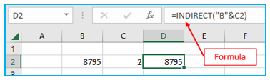
According to the following logical sequence, the formula =INDIRECT(“B”&C2) in the example below returns a value from cell B2:

The value in cell C2 is number 2, which refers to cell B2, and the INDIRECT function concatenates the components in the ref_text parameter. The formula then accesses cell B2 and returns its value, which is number 8795.

• Using the INDIRECT function with named ranges

The Excel INDIRECT function also allows you to refer to specified ranges in addition to making references from cell and text values.

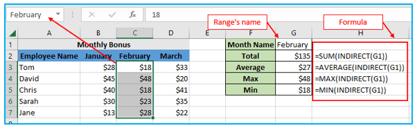
Suppose in your sheet, you have the following named ranges:

• January- B3:B7
• February – C3:C7
• March- D3:D7

Simply enter the name of the range in a cell, such as G1, and use the indirect formula =INDIRECT to refer to that cell in Excel to generate a dynamic reference to any of the aforementioned specified ranges (G1).

And now, you can go one step further and embed this INDIRECT formula into other Excel functions to determine the maximum/minimum value within the range or to calculate the sum and average of the data in a specific specified range:

=SUM(INDIRECT(G1))

=AVERAGE(INDIRECT(G1))

=MAX(INDIRECT(G1))

=MIN(INDIRECT(G1))

Once you have a general understanding of how to use Excel’s INDIRECT function, we may experiment with stronger formulas.

• INDIRECT formula that dynamically references a different worksheet

The Excel INDIRECT function is handy for more than just creating “dynamic” cell references. Here’s how you can use it to “on the fly” refer to cells in other workbooks.

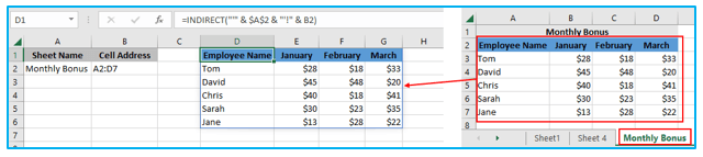
Let’s say you wish to take some crucial information from Section 4’s “Monthly Bonus” sheet into Sheet 5. An example of how an Excel Indirect formula can handle this task is shown in the screenshot below:

Let’s dissect and comprehend the formula you can see in the screenshot.

As you are aware, in Excel, references to other sheets are often made by writing the name of the sheet, an exclamation point, and a cell or range reference, such as SheetName!Range. A sheet name frequently contains a space or spaces, therefore, to avoid an error, you should better enclose it (the name, not a space:) in single quotes, for example, “Monthly Bonus!” $A$2.

Now all you have to do is combine the sheet name and cell address into a text string, feed that string to the INDIRECT function, and insert the sheet name in one cell and the cell address in another. Keep in mind that while creating a text string, you must use double quotes to contain all components other than cell addresses and numbers and the concatenation operator to connect all elements (&).

In light of the aforementioned, the following pattern emerges:

=INDIRECT(“‘” & Sheet’s name & “‘!” & Cell to pull data from)

Referring back to our example, you input the cell addresses in column B after typing the sheet’s name in cell A1 as shown in the screenshot above. The formula that results is as follows:

=INDIRECT(“‘” & $A$2 & “‘!” & B2)

Please remember to lock the reference to the sheet’s name using absolute cell references, such as $A$2, if you are copying the formula into many cells. 

Notes:

Your indirect formula will produce an error if either of the cells (A2 or B2 in the formula above) that carry the name and cell address of the second sheet are empty. This can be avoided by enclosing the INDIRECT function in the IF function:

=IF(OR($A$2=””,B2=””), “”, INDIRECT(“‘” & $A$2 & “‘!” & B2))

The referred sheet must be open for the INDIRECT formula to function properly; otherwise, the formula will produce a #REF error. Use the IFERROR method to bypass the error, which will display an empty string regardless of the error:

=IFERROR(INDIRECT(“‘” & $A$2 & “‘!” &B2), “”)

• Using INDIRECT with other Excel functions:

In addition to SUM, other Excel functions including ROW, COLUMN, ADDRESS, VLOOKUP, and SUMIF are frequently combined with INDIRECT.

• Example 1- INDIRECT and ROW functions:

The ROW function in Excel is frequently used to return an array of values. The following array formula, for instance, can be used to return the average of the three smallest numbers in the range A1:A8, but keep in mind that you must hit Ctrl + Shift + Enter.

=AVERAGE(SMALL(A1:A8,ROW(1:3)))

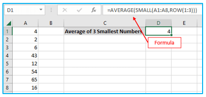
However, if you add a new row to your worksheet anywhere between rows 1 and 3, the ROW function’s range will change to ROW(1:4), and the formula will no longer return the average of the first three numbers but instead will return the average of the four smallest integers.

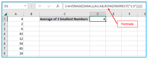
No matter how many rows are added or removed, your array formula will always be right if you nest INDIRECT in the ROW function.

=AVERAGE(SMALL(A1:A8,ROW(INDIRECT(“1:3”))))

• Example 2- Combination of INDIRECT, ADDRESS, COLUMN and ROW functions

In this example, two functions will be combined, which is a little challenging. So, let’s turn a smaller table so we may concentrate on the formula more clearly.

Let’s say you have data in 5 rows (1-5) and 4 columns (A-D):

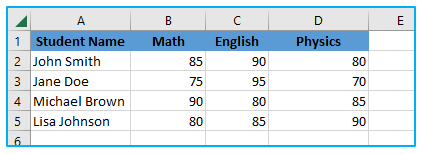
Do the following to convert columns to rows:

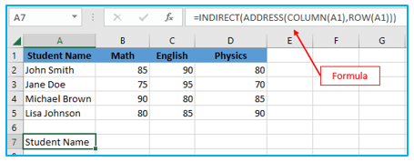
Step 1: In the leftmost cell in the target range, let’s say A7, type the following formula and press the Enter key:

=INDIRECT(ADDRESS(COLUMN(A1),ROW(A1)))

Step 2: Drag the small black cross in the lower right corner of the chosen cells to copy the formula upward and downward to as many rows and columns as necessary. All done! All of the columns in your newly constructed table have been changed to rows.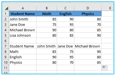

2. Excel OFFSET function – syntax and arguments

A cell or range of cells that is a specified number of rows and columns away from a specified cell or range is returned by Excel’s OFFSET function.

The Excel OFFSET formula has the following syntax:

=OFFSET(reference, rows, cols, [height], [width])

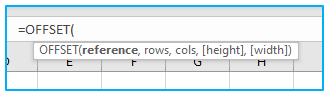
The last two parameters are optional, whereas the first three are necessary. Any of the parameters may be a cell reference or a result from another formula.

The names of the options appear to have been given some thought by Microsoft, and they do provide a suggestion as to what you should specify for each.

Required arguments:

reference – a cell or group of cells that are next to it that you base the offset on. It can be seen as the beginning.

rows – the number of rows to move up or down from the starting position. The formula advances below the initial reference if rows is a positive number, and above the starting reference if rows is a negative number.

cols – how many columns the formula should travel from its initial place. Cols can be positive (to the right of the beginning reference) or negative in addition to rows (to the left of the starting reference).

Optional arguments:

height – how many rows to return.

width – the number of returned columns

The arguments for height and width must always be positive integers. The default value is the height or width of the reference if either is absent.

The volatile function OFFSET can cause your worksheet to run slowly. The amount of cells that need to be recalculated directly relates to how sluggish it is.

Let’s now use an instance of the most basic OFFSET formula to demonstrate the principle.

• How to use OFFSET function in Excel – formula examples

I hope all that theory didn’t make you bored. Anyway, the most interesting part is now here, the actual applications of the OFFSET function in Excel.

• Excel OFFSET and SUM functions:

The use of OFFSET & SUM is most simply illustrated by the example we will cover in the next section. Let’s now examine these functions from a different perspective to discover what else they are capable of.

• Example 1- A SUM/OFFSET formula that is dynamic:

You might require an SUM formula that automatically selects all newly added rows while working with worksheets that are regularly updated.

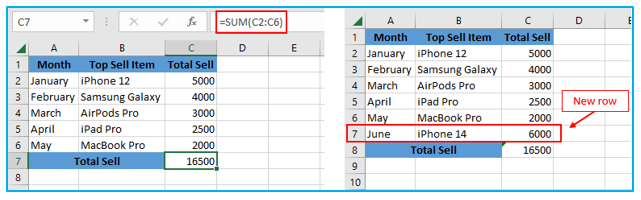
Assume that your source data looks something like the screenshot shown below. A new row is created each month just above the SUM formula, and you obviously want it to be included in the total. In general, you have two options: manually adjust the range in the SUM formula each time or let the OFFSET formula take care of it.

You simply need to choose the parameters for the Excel OFFSET function, which will get that last cell of the range, as the first cell of the range to sum will be directly stated in the SUM formula:

Reference – The whole cell, which in our situation is C8.

Rows – The cell that needs the negative number -1 is the one just above the total.

Cols – Since you don’t wish to change the column, it is zero.

The SUM/OFFSET formula pattern is as follows:

=SUM(first cell:(OFFSET(cell with total, -1,0)

For the aforementioned case, the formula is modified to look like this:

=SUM(C2:(OFFSET(C8, -1, 0)))

And it operates perfectly, as shown in the screenshot below: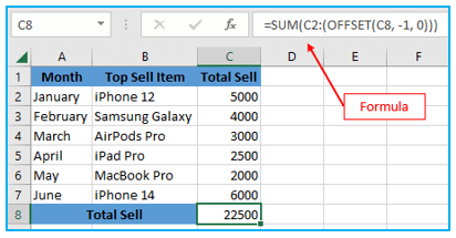

• Example 2- To sum the last N rows in Excel, use the OFFSET formula:

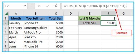
Assume that instead of the overall total in the example above, you would like to know the total amount of sales for the last N months. Additionally, you want the formula to automatically include any additional rows you insert into the sheet.

We will combine the Excel OFFSET function with the SUM, COUNT, and COUNTA functions to complete this task:

=SUM(OFFSET(C1,COUNT(C:C)-F1+1,0,F1,1))

Or

=SUM(OFFSET(C1,COUNTA(C:C)-F1,0,F1,1))

You can better comprehend the formulas by knowing the information below:

Reference: In this example, cell C1 is the heading of the column whose values you want to total.

Rows: You can use the COUNT or COUNTA function to determine how many rows need to be offset.

After subtracting the most recent N months (the number is in cell F1) and adding 1, COUNT returns the number of cells in column B that contain numbers.

Since COUNTA counts all non-empty cells and a header row with a text value provides an additional cell that our formula needs, you don’t need to add 1 if COUNTA is your preferred function. Please be aware that this formula will only function properly on tables with a similar layout—a header row, followed by rows with numbers. You might need to modify the OFFSET/COUNTA formula for various table layouts.

Cols – There are no more columns to offset (0).

Height – F1 states how many rows should be added.

Width – 1 column.

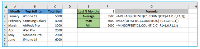
• Using OFFSET function with AVERAGE, MAX, MIN:

You can obtain the average of the last N days, weeks, or years as well as their highest or minimum values in the same way that we computed the total sales for the previous N months. The first function’s name is the only distinction between the formulas:

=AVERAGE(OFFSET(C1,COUNT(C:C)-F1+1,0,F1,1))

=MAX(OFFSET(C1,COUNT(C:C)-F1+1,0,F1,1))

=MIN(OFFSET(C1,COUNT(C:C)-F1+1,0,F1,1))

You won’t need to alter the formula each time your source table is updated, which is a major advantage over the standard AVERAGE(C5:C7) or MAX(C5:C7). Your worksheet’s OFFSET formulae will always refer to the set number of last (lower-most) cells in the column, regardless of how many additional rows are added or subtracted from it.

• Making a dynamic range with Excel’s OFFSET formula

The COUNTA function counts the number of cells in a range of cells while eliminating any empty cells. We will now assign the row height and column width based on the data present in the range using COUNTA functions.

Step 1: Choose Cell G1 and type the formula below:

=OFFSET(A1,0,0,COUNTA(A:A),COUNTA(A1:D1))

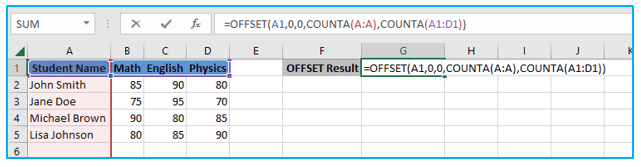
Step 2: When you hit Enter, the entire array will appear as the resultant values.

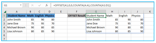
The COUNTA(A:A) function was used in the argument section to assign the row height, which means we are allocating the rows up to the maximum row in the spreadsheet so that any new values entered under the initial range of data in the row would also be saved by the OFFSET function. The four columns (A, B, C, and D) are now assigned to the function based on the reference value chosen in the OFFSET function because the column width has once again been defined as COUNTA(A1:D1).

• Excel OFFSET & VLOOKUP

Everyone is aware that the VLOOKUP or HLOOKUP functions may be used to conduct straightforward vertical and horizontal lookups, respectively. These functions, however, have too many restrictions and frequently falter in increasingly potent and intricate lookup formulas. Therefore, you must explore for alternatives like INDEX, MATCH, and OFFSET in order to do more complex lookups in your Excel tables.

• Example 1-Vlookup left in Excel using the OFFSET formula

The inability of the VLOOKUP function to look to its left, or to return a value other than that to the right of the lookup column, is one of its most well-known limitations.

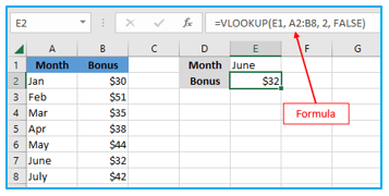
Month names (column A) and bonuses are the two columns in our sample lookup table (column B). This straightforward VLOOKUP formula will function without a hitch if you wish to receive a bonus for a specific month:

=VLOOKUP(E1, A2:B8, 2, FALSE)

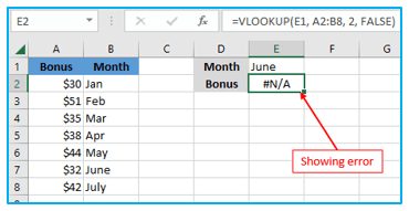
However, as soon as you switch the columns in the lookup table, the #N/A error will appear:

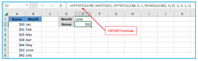
You need a more adaptable function that doesn’t really care where the return column is located to accommodate a left-side lookup. Using the INDEX and MATCH functions in conjunction is one solution that might be used. The use of OFFSET, MATCH, and ROWS is another strategy:

=OFFSET(lookup_table, MATCH(lookup_value, OFFSET(lookup_table, 0, lookup_col_offset, ROWS(lookup_table), 1) ,0) -1, return_col_offset, 1, 1)

Where:

Lookup_col_offset – is how many columns need to be moved from the origin to the lookup column.

Return_col_offset – which represents how many columns must be moved to get from the origin to the return column.

In our example, the lookup table is A2:B8, the lookup value is in cell E1, the lookup column offset is 1 (we need to move 1 column to the right from the beginning of the table in order to find the lookup value in the second column (B), and the return column offset is 0 because we are returning values from the first column (A)) and the return column offset is 0.

=OFFSET(A2:B8, MATCH(E1, OFFSET(A2:B8, 0, 1, ROWS(A2:B8), 1),0) -1, 0, 1, 1)

Although the formula appears awkward, it actually works.

• Example 2- Two-way lookup (by column and row values):

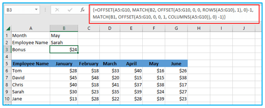
A value from a two-way lookup is based on matches in both the rows and columns. Additionally, you can get a value at the point where a specific row and column meet by using the double lookup array formula shown below:

=OFFSET(lookup table, MATCH(row lookup value, OFFSET(lookup table, 0, 0, ROWS(lookup table), 1), 0) -1, MATCH(column lookup value, OFFSET(lookup table, 0, 0, 1, COLUMNS(lookup table)), 0) -1)

Given that:

• A5:G10 is the lookup table.
• B2 has the matching value for the rows.
• The column’s matching value is in B1

The two-dimensional lookup formula is as follows:

=OFFSET(A5:G10, MATCH(B2, OFFSET(A5:G10, 0, 0, ROWS(A5:G10), 1), 0)-1,

MATCH(B1, OFFSET(A5:G10, 0, 0, 1, COLUMNS(A5:G10)), 0) -1)

It’s not the most straightforward thing to recall, is it? Additionally, as this is an array formula, remember to input it correctly by pressing Ctrl + Shift + Enter.

Of course, there are other ways to perform a double lookup in Excel than the lengthy OFFSET formula. The VLOOKUP & MATCH, SUMPRODUCT, or INDEX & MATCH operations will all produce the identical outcome. Even without using a formula, named ranges and the intersection operator can be used (space).

• Limitation of OFFSET Function

The examples of formulas on this page should have clarified how to utilize OFFSET in Excel. However, in order to effectively use the function in your own workbooks, you should be aware of both its advantages and disadvantages.

The following are the Excel OFFSET function’s most significant restrictions:

1. OFFSET is a resource-hungry function, just like other volatile functions. Your OFFSET formulas are updated whenever there is a change in the source data, which keeps Excel busy for a little while longer. For a single formula on a small spreadsheet, this is not a problem. However, Microsoft Excel could take a while to recalculate if a workbook has dozens or even hundreds of formulas.
2. It’s difficult to review Excel OFFSET formulas. Big formulas (particularly with nested OFFSETs) might be difficult to debug since references returned by the OFFSET function are dynamic.

• Alternatives to using OFFSET in Excel

The same result can be obtained in a variety of different ways, as is frequently the case in Excel. So, here are three classy substitutions for OFFSET.

Excel tables:

Fully-fledged Excel tables, as opposed to standard ranges, have been available since Excel 2002, and they are a genuinely amazing feature. Simply select Table from the Insert menu under the Home tab or press Ctrl + T to create a table from structured data.

An Excel table can be made into a “calculated column” by writing a formula in one cell, which then automatically duplicates the formula to all other cells in that column and modifies it for each row in the table.

Additionally, any formula that uses a table’s data will immediately be adjusted to include or exclude any new rows you add or delete. Technically, these formulas work with the dynamic ranges that make up the columns and rows of tables. You can rename your table using the Design tab > Properties group > Table Name text box. Each table in a workbook has a distinct name (the defaults are Table1, Table2, etc.).

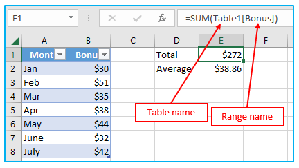
The SUM calculation that uses Table 1’s Bonus column is seen in the screenshot below. Please note that the formula uses the column name from the table rather than a set of cells.

INDEX function in Excel

The Excel INDEX function can also be used to construct dynamic range references, albeit not precisely in the same way as OFFSET. The INDEX function is not volatile, unlike OFFSET, thus it won’t cause Excel to lag.

INDIRECT function in Excel

You can construct dynamic range references from a variety of sources, including cell values, cell values and text, and specified ranges, by using the INDIRECT function. Additionally, it can dynamically refer to another Excel file or sheet. These formula examples can be found in our Excel INDIRECT function tutorial.

Application of Excel INDIRECT Function and Excel OFFSET Function

Excel INDIRECT Function:

• Dynamic Cell Reference: Use INDIRECT to create a cell reference based on text strings, enabling dynamic changes to formulas without altering the formula itself.
• Combining Multiple Sheets: Create summary reports by referring to cell values across different sheets using INDIRECT, facilitating consolidated data analysis from various sources.
• Data Validation Lists: Employ INDIRECT in data validation to create dependent dropdown lists where the selection in one list determines the options in another.
• Conditional Summing Across Tabs: Sum data across multiple tabs based on specific conditions by combining INDIRECT with SUMIF or SUMIFS functions, enhancing flexibility in data aggregation.
• Creating Flexible Ranges: Utilize INDIRECT to construct flexible range references within formulas like SUM or AVERAGE, allowing the range to adapt when new data is added or removed.
• Dynamic Named Ranges: Define named ranges that can adjust dynamically by using INDIRECT, making your named ranges more adaptable to changes in data size.

Excel OFFSET Function:

• Dynamic Range Selection: Use OFFSET to select different data ranges dynamically based on specified parameters, ideal for creating dynamic charts or analyzing varying data sets.
• Creating Rolling Averages: Calculate rolling or moving averages by using OFFSET to shift the average range through time or data points, useful for trend analysis.
• Conditional Data Extraction: Extract specific data from a larger set based on certain conditions by combining OFFSET with MATCH or other lookup functions, tailoring data retrieval to specific needs.
• Automating Data Summarization: Summarize data automatically by defining a range with OFFSET that expands or contracts based on criteria, streamlining data compilation tasks.
• Adjusting to Data Growth: Accommodate growing datasets by using OFFSET to refer to expanding or contracting ranges in formulas, ensuring calculations remain accurate over time.
• Variable Data Table Creation: Generate data tables with varying parameters by using OFFSET to alter the range and scope of table data, aiding in scenario analysis and sensitivity testing.

For ready-to-use Dashboard Templates:

1. Financial Dashboards
2. Sales Dashboards
3. HR Dashboards
4. Data Visualization Charts