IFERROR in Excel is a game-changer for data enthusiasts seeking seamless spreadsheet experiences. This powerful function is designed to streamline your workflow by handling errors gracefully, ensuring your calculations remain uninterrupted and your data presentation is impeccable. In this comprehensive guide, we delve into the nuances of the IFERROR function, teaching you how to effectively manage and mitigate common error pitfalls in Excel. Embrace the full potential of IFERROR and elevate your data analysis to new heights of precision and professionalism.
The lesson demonstrates how to utilize Excel’s IFERROR function to detect problems and replace them with blank cells, different values, or personalized messages. You’ll discover how to use the IFERROR function in conjunction with Vlookup and Index Match as well as how it differs from IF ISERROR and IFNA.
This Tutorial Covers:
- What is IFERROR in Excel
- How to use IFERROR in Excel – formula examples
- IFERROR VLOOKUP formula
- Nested IFERROR Functions
- IFERROR in array formulas
- IFERROR vs. IF ISERROR
- IFERROR vs. IFNA
1. What is IFERROR in Excel?
For the purpose of managing and catching errors in formulas and calculations, Excel has a function called IFERROR. IFERROR explicitly tests a formula and, if it evaluates an error, returns a different value you specify; otherwise, it returns the calculation’s outcome.
The Excel IFERROR function has the following syntax:
IFERROR(value, value_if_error)
Where:
value (required)- How to check for mistakes. It might be an expression, formula, value, or cell reference.
value_if_error (required)- what to return if a mistake is discovered. It could be a blank cell, text message, numeric value, formula, or other calculation. It could also be an empty string.
For instance, if one of the columns contains empty cells, zeros, or text, you can receive a variety of problems while dividing two columns of integers.
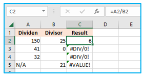
Use the IFERROR Excel function to identify and manage errors as you see fit to avoid that from occurring.
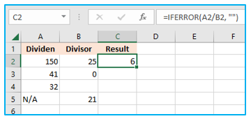
If error, then blank
To return a blank cell if an error is encountered, pass the value if error option an empty string (“):
=IFERROR(A2/B2, “”)
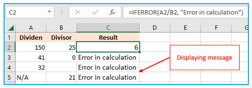
If error, display a message
In addition, you can substitute your own message for Excel’s default error notation:
=IFERROR(A2/B2, “Error in calculation”)
The Excel IFERROR function: 5 things to know:
- All error kinds, including #DIV/0!, #N/A, #NAME?, #NULL!, #NUM!, #REF!, and #VALUE!, are supported by Excel’s IFERROR function.
- IFERROR can substitute errors with your personalized text message, a number, a date, a logical value, the outcome of another formula, or an empty string depending on the contents of the value if error parameter (blank cell).
- It is not considered a mistake if the value argument is a blank cell, but it is regarded as an empty string (“‘).
- The quick option to use the IFERROR function in Excel was first made accessible in Excel 2007 and has since been included in Excel 2010, 2013, 2016, 2019, and Excel 2021 as well as Excel 365.
- Use the ISERROR function along with IF, as seen in this example, to catch mistakes in Excel 2003 and prior versions.
2. How to use IFERROR in Excel – formula examples:
The examples that follow demonstrate how to utilize IFERROR in Excel in conjunction with other functions to carry out more challenging tasks.
- IFERROR VLOOKUP formula:
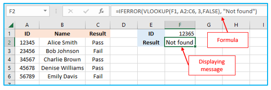
Informing users that a value they are looking for doesn’t exist in the data set is one of the most popular uses of the IFERROR function. To achieve this, you would wrap a VLOOKUP formula with IFERROR like follows:
=IFERROR(VLOOKUP(…),”Not found”)
A standard Vlookup formula would return the #N/A error if the lookup value was not present in the table you were searching for in.
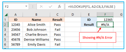
How to use IFERROR function in excel is shown below:
Wrap VLOOKUP in IFERROR and present a more detailed and user-friendly warning to give your users peace of mind:
=IFERROR(VLOOKUP(A2, ‘Lookup table’!$A$2:$B$4, 2,FALSE), “Not found”)
This Excel formula for IFERROR is displayed in the screenshot below:
- Nested IFERROR Functions:
What is nested IFERROR Function?
To conduct several lookups sequentially, one or more VLOOKUP formulas may be nested inside another VLOOKUP calculation. IFERROR detects the problem and executes the second VLOOKUP function if the first VLOOKUP fails. The error message that is given in the formula is printed if that too fails. If not, the function’s output is returned.
You can stack two or more IFERROR functions one inside the other when you need to execute additional VLOOKUP dependent on whether the prior Vlookup was successful or unsuccessful.
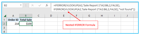
Suppose you want to get the amount for a specific order ID, and you have a number of sales reports from your company’s regional offices.

How to use nested IFERROR function is shown below:
Step 1: Enter the formula as follows in cell B2, using A2 as the lookup value in the current sheet and A2:B6 as the lookup range in three lookup sheets (Sale Report 1, and Sale Report 2).
=IFERROR(VLOOKUP(A2,’Sale Report 1′!A2:B6,2,FALSE),IFERROR(VLOOKUP(A2,’Sale Report 2′!A2:B6,2,FALSE),”not found”))
The outcome will resemble something like this:
- IFERROR in array formulas:
Array formulae in Excel, as you are surely aware, are designed to carry out several calculations within a single formula. The IFERROR function will return an array of values for each cell in the specified range if you supply an array formula or expression as the value parameter. Details are displayed in the sample below.
Let’s say you want to calculate “Total Quantity” and you have “Item Name” in column A, “Total Price” in column B, and “Price” in column C.
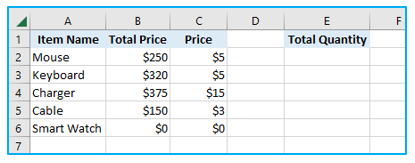
This can be accomplished by dividing each cell in the range B2:B6 by its corresponding cell in the range C2:C6, adding the results, and then using the array formula shown below:
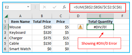
=SUM($B$2:$B$6/$C$2:$C$6)
As long as the divisor range contains no zeros or empty cells, the formula is valid. The #DIV/0! error is displayed if at least one cell has a value of 0 or is blank:
Simply perform the division within the IFERROR function to correct the error:
=SUM(IFERROR($B$2:$B$6/$C$2:$C$6,0))
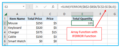
The formula produces the array of results 50; 64; 25; 50; #DIV/0! by dividing a value in column B by a value in column C in each row (250/5, 320/5, 375/15, 150/3, and 0/0). All #DIV/0! errors are caught by the IFERROR function, which substitutes them with zeros. The final result (50+64+25+50=189) is then printed by adding the values in the resultant array, which are 50, 64, 25, 50, and 0.
Note: Please keep in mind that the shortcut Ctrl + Shift + Enter should be used to finish array formulas.
3. IFERROR vs. IF ISERROR:
You might be wondering why some people still choose to utilize the IF ISERROR combination after learning how simple it is to use the IFERROR function in Excel. Does it offer any benefits over IFERROR? None. When IFERROR was not available in Excel 2003 and earlier IF ISERROR was the sole method that could be used to catch mistakes. It’s simply a little bit trickier in Excel 2007 and later to get the same effect.
For instance, you can use either of the algorithms below to detect Vlookup issues.
In Excel 2007 – Excel 2021:
=IFERROR(VLOOKUP(…), “Not found”)
In all Excel versions:
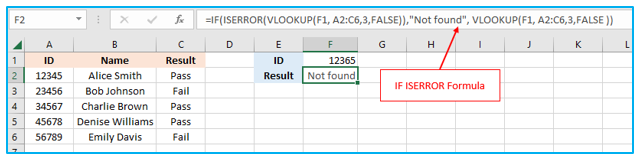
=IF(ISERROR(VLOOKUP(…)), “Not found”, VLOOKUP(…))
You should be aware that you must Vlookup twice in the IF ISERROR VLOOKUP formula. The formula can be interpreted as follows in simple English: If Vlookup fails, it should return “Not found,” but if it succeeds, it should print the result.
The following is an actual Excel IF ISERROR Vlookup formula example:
=IF(ISERROR(VLOOKUP(F1, A2:C6,3,FALSE)),”Not found”, VLOOKUP(F1, A2:C6,3,FALSE ))
4. IFERROR vs. IFNA:
IFNA is an additional function to check a formula for mistakes that were included with Excel 2013. Its syntax is comparable to IFERROR’s:
IFNA(value, value_if_na)
What distinguishes IFNA from IFERROR? Only #N/A errors are caught by the IFNA function, whereas all error kinds are handled by IFERROR.
What circumstances could you wish to employ IFNA? when it is bad practice to hide all mistakes. When working with sensitive or critical data, for instance, you might want to be alerted to potential errors in your data collection; in this case, typical Excel error alerts with the “#” symbol could serve as clear visual cues.
Let’s look at how to create a formula that highlights additional Excel problems while displaying the “Not found” message rather than the N/A error, which happens when the lookup value is missing from the data collection.
As seen in the screenshot below, let’s say you wish to transfer Qty. from the lookup table to the summary table. Although the Excel IFERROR VLOOKUP formula might result in a visually appealing output, “Charger” do exist in the lookup database, hence the result is technically incorrect:
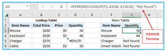
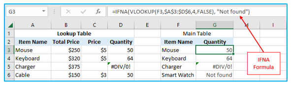
In Excel 2013 and Excel 2016, use the IFNA function to detect #N/A but show the #DIV/0 error:
=IFNA(VLOOKUP(F3,$A$3:$D$6,4,FALSE), “Not found”)
Or, in Excel 2010 and older versions, use the IF ISNA combination:
=IF(ISNA(VLOOKUP(F3,$A$3:$D$6,4,FALSE)),”Not found”, VLOOKUP(F3,$A$3:$D$6,4,FALSE))
The syntax of the previously disclosed IFERROR VLOOKUP and IF ISERROR VLOOKUP formulae is shared by the IFNA VLOOKUP and IF ISNA VLOOKUP formulas.
The IFNA VLOOKUP formula only returns “Not found” for items that are absent from the lookup table, as seen in the screenshot below (Smart Watch). The display for Charger is #DIV/0. demonstrating that a divide by zero error exists in our lookup table:
Some of the benefits of the IFERROR function are listed below:
- All error kinds, including #NULL!, #REF!, #DIV/0!, #NUM!, #VALUE!, #NAME?, and #N/A, are handled by the Excel IFERROR function.
- Depending on the contents of the value if error aspect, IFERROR can replace errors with customer numeric values, dates, the output of other formulas, or text.
- Your value parameter will be handled as an empty string rather than an error if it is empty.
Excel 2007 marked the debut of the IFERROR function, which has remained accessible ever since.
You may be interested:
