DSUM Function in Excel is a powerful tool for data analysis, offering precise calculations based on specified criteria. With its ability to dynamically update calculations and handle multiple criteria, DSUM enhances the accuracy and efficiency of data analysis tasks. By seamlessly integrating with other Excel functions and features, it facilitates comprehensive analysis and decision-making processes. Whether you’re summarizing data, performing conditional summing, or validating entries, DSUM Function in Excel provides the flexibility and reliability needed for effective data analysis. Unlock the full potential of your Excel spreadsheets with DSUM Function in Excel today.
- What is the DSUM Function?
- How to use the DSUM Function in Excel?
- Understanding the syntax of the DSUM function in Excel.
- Calculate the revenue with the help of DSUM function.
- Things you should remember about DSUM function.
1. What is the DSUM Function?
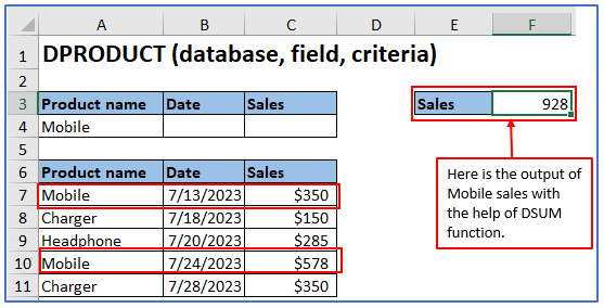
In Excel, the DSUM function is also called its own: DATABASE SUM. By utilizing specific fields and criteria, the totals for the specific database can be determined. Three inputs are used in the function: a database range, corresponding fields, and conditions. The total value of the matching records to the criteria is returned by the Excel DSUM function.
The summaries are obtained from fields in the database that are not included.
2. How to use the DSUM Function in Excel?
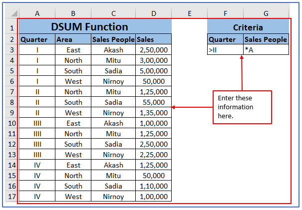
Step 1: Suppose you have obtained sales data. You want to find the sales of all salespeople whose names begin with the letter A. Here used A* to examine the numbers.
The specified criteria are: Quarter: >II
Salesperson: *A. Enter the data and criteria into the excel sheet.
Entered the data here.
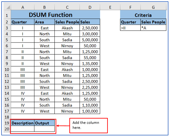
Step 2: Now, add the column in A19,A20 and B19, B20 to get the DSUM result there.
The column has been added.
Step 3: Now, use the formula of DSUM function to find the sales of all salespeople whose names begin with the letter A. The formula is: =DSUM(A3:D17,4,F2,G3). The field argument has a number instead of “Sales” (to indicate the fourth) 4 was used database columns).
Applied the formula here.
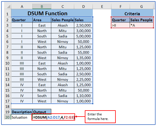
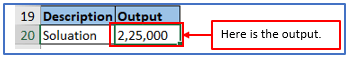
Step 4: Sales people beginning with the letter A are recorded in DSUM for all sales made since Q2 by these Sales people.
The result is $2,25,000.
3. Understanding the syntax of the DSUM function in Excel.
Syntax: DSUM(database, field, criteria)
The syntax has the following arguments:
Database: A set of individual cells that constitutes a list or database. A database consists of a list of related data, with records in the rows and fields in columns. Each column’s labels are arranged in the first row of the list.
Field: Specifies the columns used in the function. Enter a column label with double quotes, such as “Age” or “Yield,” or enter a number (without quotes) to indicate the column’s position in the list: 1, 2 for the first column. 2, and so on in the second column.
Criteria: Several cells that exhibit the mentioned phenomenon. The criteria argument can have any range as long as it has a column label and criterion for the column.
4. Calculate the revenue with the help of DSUM function.
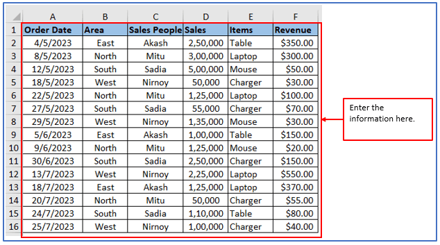
Step 1: Organize the data, and make a table into the excel sheet.
Placed the information here.
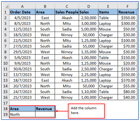
Step 2: Choose the column in A18:A19 and B18:B19 to get the north area sales revenue there as instructed below.
The column has been added.
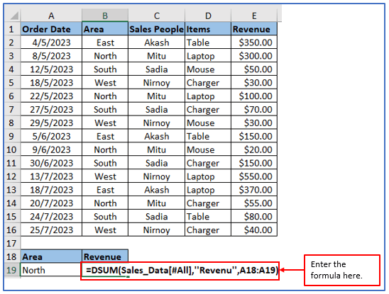
Step 3: Now, use the formula of DSUM function to find the North area sales revenue. The formula is: =DSUM(Sales_Data[#All],”Revenu”,A18:A19) . Here, you need to specify the “North” area as the criterion. Indicates which columns should be summed “Revenue” column in the table. Occupies database space, the database “Sales_Data”.
Applied the formula here.
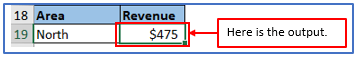
Step 4: Here is the revenue of North area.
The revenue is $475.00
5. Things you should remember about DSUM function.
- When writing the field name, it must be enclosed in double quotes and must be the same as the table header.
- Determine the necessary conditions and enumerate all prerequisites.
- A table must be created for the data. Large data sets are referred to as ranges when it becomes large. You don’t need to worry about range.
- #Value error is caused by an incorrect field name in the database argument.
- If you do not specify any specific criteria, only the column sum is retrieved.
- Creating a list of conditions that can be used to determine the different regions or number of repeats is necessary.
- If you change the dropdown list, thee-sensitive the results may be displayed accordingly. Criteria tables are not case sensitive.
- Alternative expressions for the SUMIF and SUMIFS functions. You can use SUMIFS to match multiple conditions and add any range of data, much like Excel’s SUMIF formula.
Application of DSUM Function in Excel
- Summarize Data: DSUM function calculates the sum of values in a database based on specified criteria.
- Dynamic Summation: It dynamically updates calculations as new data is added or modified in the database.
- Conditional Summing: Allows for summing only those records that meet specific criteria, providing flexibility in analysis.
- Multiple Criteria: DSUM function can handle multiple criteria, enabling complex filtering and analysis of data.
- Integration with Excel Features: Integrates seamlessly with other Excel functions and features for comprehensive data analysis.
- Data Validation: DSUM function ensures accuracy by validating data entries against defined criteria before performing calculations.
You may be interested:
