The DELTA function in Excel is a useful tool for testing whether two values are equal. With this function, you can quickly determine if two values are the same, and return a value of 1 if they are, and 0 if they are not. In this tutorial, we’ll cover the basics of how to use the DELTA function in Excel, including its syntax and some examples to help you get started.
This Tutorial Covers:
- What is DELTA function in Excel
- Syntax of DELTA function in Excel
- Arguments of DELTA function in Excel
- Using DELTA Function in Excel
- Example 1- Find Similar Values Between Two Columns Through DELTA Function
- Example 2- Insert DELTA Function to Compare Column Values with 0
- Example 3- Utilize DELTA Function to Determine Number Format in Excel
- Remarks
1. What is DELTA function in Excel?
The DELTA function in Excel is a logical function that compares two values and returns a result of 1 if the values are equal, and 0 if they are not. The function is particularly useful when you need to test whether two values are equal before performing a specific action, such as in conditional formatting or complex calculations. The DELTA function is available in most versions of Excel, including Excel 2010, Excel 2013, Excel 2016, and Excel 2019.
- Syntax of DELTA function in Excel:
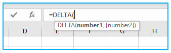
The Excel DELTA function’s syntax is quite basic and easy to understand. It has the following structure:
=DELTA(number1, [number2])
- Arguments of DELTA function in Excel:
The following arguments are part of the DELTA function syntax:
number1 (required): the first number you want to compare.
number2 (optional): The second number you want to compare. Excel will presume the value to be zero if this argument is left out.
2. Using DELTA Function in Excel:
In this tutorial, we will explore the use of the DELTA function in Microsoft Excel 365. To illustrate its practical applications, we will analyze the sample dataset below. Whether you are using Excel 365 or another version, the concepts discussed in this post can be applied in a similar manner.

- Example 1- Find Similar Values Between Two Columns Through DELTA Function:
We will explore the first example of using the Excel DELTA function, which involves finding similar values in two columns. For this purpose, we will compare the marks of two students using the DELTA function in Excel. The function returns a value of 1 in the Result column if the marks are identical, and 0 if they are not. To make it easier to understand the results, we will use the IF function in conjunction with the DELTA function.
To follow along with this example, please read and follow the instructions carefully:
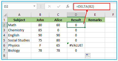
Step 1: Apply the below formula in cell D2 and you can either copy and paste the formula or drag the formula’s fill handle to the remaining cells.
=DELTA(B2,C2)
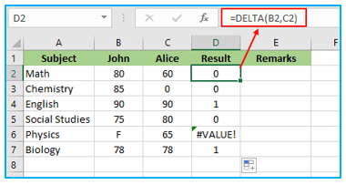
Because one of our values is not a numeric, we discover a VALUE# error in cell D6. F in cell B6 in this instance.
Apply the formula shown below in cell E2 at this point. You can then copy and paste the formula or drag the fill handle of the formula to the remaining cells.
=IF(D2=1,”Same”,”Different”)
Finally, we can see our desired output down below.
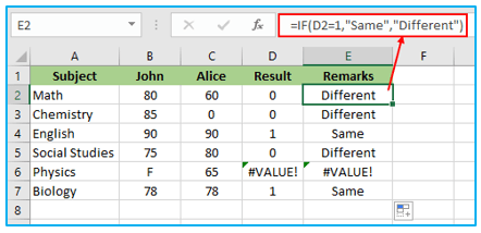
Another VALUE# mistake will occur in E6 as a result of the D6 cell.
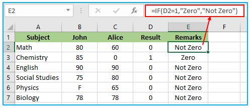
- Example 2- Insert DELTA Function to Compare Column Values with 0
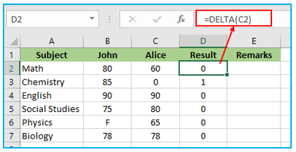
In the second example of using the DELTA function in this tutorial, we will compare cell values with zero. Specifically, we will use the DELTA function to compare Alice’s mark in column C with zero. In this case, we only need to provide the Required parameter of the DELTA function, as the optional parameter is assumed to be zero if it is not provided. To better understand the results, we will again use the IF function to illustrate a remark.
To complete this example, please follow the instructions carefully:
Step 1: Apply the below formula in cell D2 and you can either copy and paste the formula or drag the formula’s fill handle to the remaining cells.
=DELTA(C2)
Apply the formula shown below in cell E2 at this point. You can then copy and paste the formula or drag the fill handle of the formula to the remaining cells.
=IF(D2=1,”Zero”,”Not Zero”)
Finally, we can see our desired output down below.
- Example 3- Utilize DELTA Function to Determine Number Format in Excel:
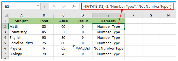
In addition to the previous examples, we will now explore another practical use case of the DELTA function. We can use the function to determine if the value in a cell is a number or not. For this example, we will use the DELTA function to check if the values in columns B and C are numeric. To further illustrate the results, we will use the TYPE function to display a message in the Remarks column.
To complete this example, please follow the instructions carefully:
Step 1: Apply the below formula in cell D2 and you can either copy and paste the formula or drag the formula’s fill handle to the remaining cells.
=DELTA(B2)
The corresponding output is displayed below.
Apply the formula shown below in cell E2 at this point. You can then copy and paste the formula or drag the fill handle of the formula to the remaining cells.
=IF(D2=1,”Zero”,”Not Zero”)
Finally, we can see our desired output down below.
3. Remarks
In case the second parameter (number2) is omitted, DELTA function assumes that its value is zero.
When either of the values being compared is in a text format, DELTA function will generate an error message displaying #VALUE.
Having learned about the DELTA formula in Excel and its usage through the examples presented, you are now equipped to incorporate it into your Excel tasks.
For ready-to-use Dashboard Templates:
