The CORREL function in Excel is a powerful tool for statisticians, data analysts, and anyone keen on understanding the relationship between two sets of data. This function computes the correlation coefficient, a crucial statistic that measures the degree of linear relationship between two variables, offering insights into trends, patterns, and predictive modeling. Whether you’re in finance analyzing stock market trends, in marketing assessing consumer behavior, or in healthcare studying clinical data, this guide will navigate you through the process of using the CORREL function in Excel. By mastering this function, you’ll be able to unveil hidden relationships in your data, leading to more informed decisions and strategic planning.
This content Covers:
- What is the CORREL Function?
- What are some uses of the CORREL function in Excel?
- How to use CORREL Function in Excel?
- Some points to remember about the CORREL Function
- How to Find Correlation Coefficient in Excel?
1. What is the CORREL Function?
The CORREL function simplifies this calculation and makes it easy to find correlations between two data sets in Excel.
A correlation coefficient is a statistical measure that quantifies the strength and direction of a linear relationship between two data sets.
It is used to determine whether there is a positive or negative relationship between variables and ranges from -1 to 1.
- A value of 1 indicates a perfect positive correlation, meaning the variables move in the same direction.
- A value of -1 indicates a perfect negative correlation, meaning the variables move in opposite directions.
- Values close to 0 indicate weak or no correlation.
- There is no linear relationship between the variables.
2. What are some uses of the CORREL function in Excel?
- Portfolio management:
In here, the CORREL function is often used to evaluate correlations between different investments. By analyzing the correlation coefficient between assets or asset classes, investors can build diversified portfolios that reduce overall risk. Assets with low or negative correlation tend to move independently of each other, reducing risk more effectively.
- Forecasting and forecasting:
The CORREL function helps you make predictions and forecasts by identifying relationships between variables. By calculating correlations between historical data, you can predict future results. For example, you can predict future sales by analyzing the correlation between sales and various factors such as advertising spend, economic indicators, and seasonal trends.
- Risk analysis:
CORREL functionality is useful for risk analysis and risk management. By analyzing the correlation between variables such as market indexes and asset returns, you can assess the degree of systematic risk in your portfolio. Understanding the correlation between investments can help you identify potential vulnerabilities and make informed decisions to reduce risk.
- Data validation:
The CORREL function can be used as a data validation tool. It helps ensure data integrity by checking for errors and inconsistencies in records. Correlation coefficients outside a certain range may indicate data entry errors, outliers, or missing values that require further investigation.
3. How to use CORREL Function in Excel?
While doing Correl function in excel you have to follow a syntax that is:
=CORREL(array1, array2)
“Array1” is the first set of data values.
“Array2” is the second set of data values.
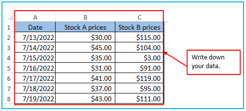
Step 1: First you need to prepare your data then organize your data into two columns or tables, where each column represents a different variable or set of data.
Now put your data into your excel sheet as shown below:
Step 2: After entering your data where you want to show the correlation you need to put in the CORREL function with the exact array.
Suppose you want to work with the data is in columns A and C same as the picture showing, for this you need to choose (A1:A8, C1:C8).

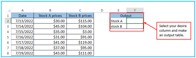
Step 3: Now you need to create another table with the results. For this choose column E so that you can get the output for Stock A and Stock B.
Step 4: Now, write down the formula for stock A =CORREL(A2:A8, C2:C8) in the Output column as shown.

Step 5: Now, do press enter Key.
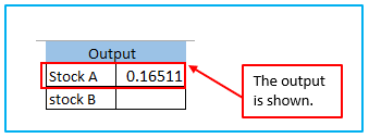
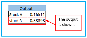
You can see the results in the output box in which Excel calculates the correlation coefficient between two data sets A2 to A8 and C2 to C8.
Now, you can use the same formula for Stock B according to your column. The formula will be: =CORREL(A2:A8,B2:B8)
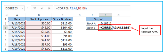
After entering the formula press Enter and you will get the result for Stock B.
The result is outlined below:
4. Some points to remember about the CORREL Function
- N/A error – When the specified arrays have different lengths that time it Occurs. Therefore, if Array1 and Array2 contain different numbers of data points, CORREL returns the error value N/A.
- DIV/0 error – Occurs when one of the specified arrays is empty or the standard deviation of their values is 0. If the array or reference argument contains text, logical values, or empty cells, the values are ignored. However, cells with a value of zero are also considered.
5. How to Find Correlation Coefficient in Excel?
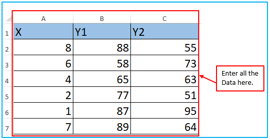
Step 1: You need to make an data table first.
Where, Put Variable array1 as X
Variable array2 as Y1 and array3 as Y2.
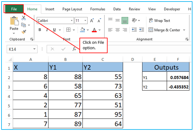
Make a table as shown below and put the data into the column.
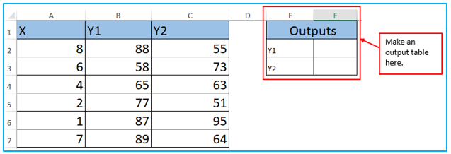
Step 2: Now make another table for finding the Correlation for Y1 and Y2.
Make a table in Columns E and F to get the Correlation of X of Y1 and X of Y2 as shown.
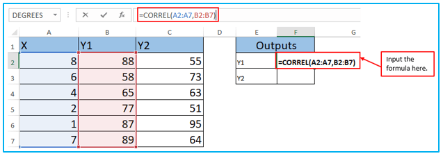
Step3: The formula for finding the Correlation of Y1 is:
=CORREL(array1,array2) or =CORREL(A2:A7,B2:B7)
array1: Set of values of X. The cell range is from A2 to A7.
array2 : Set of values of Y1. The cell range is from B2 to B7.
Now, you can follow the below formula for finding the correlation for the variables X and Y1.
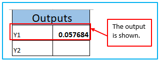
Step 4: After writing down the formula now press enter.
After pressing the enter key you will get the result of Array X and Array Y1 as shown.
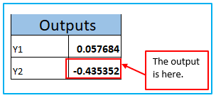
For Array X and Array Y2 you need to follow Step 2 and you will get the result it like this. For X and Y2 the formula will be: =CORREL(A2:A7,C2:C7).
Enter the formula according to your column as shown below:

After using the formula press Enter the result of X and Y2 will appear.
The result is outlined below:
Step 5: Now, Go to the file tab as shown below.
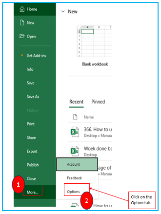
Step 6: After clicking on the file tab, You can see a home page will appear. Now, click on MORE tab and you will get an Option tab.
Do click on Option tab.
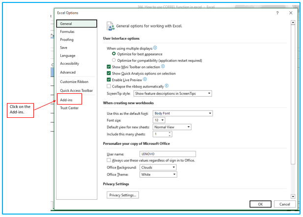
Step 7: After clicking on Option the Excel Options dialog box will open. Click on the Add-Ins option as shown below.
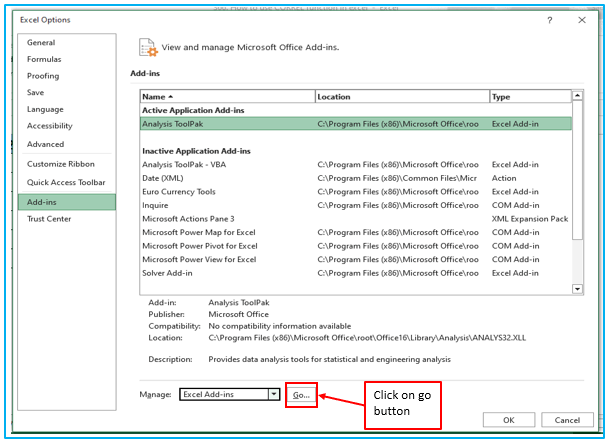
Step 8: After clicking Add-ins, you will get a page the same as like which is in the one below and then you can see Excel Add-ins from the drop-down in the Manage and click on the Go button as showing.
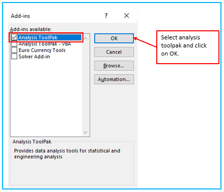
Step 9: After clicking on Go the Add-ins dialog box opens and in this option, you can see Analysis ToolPak.
Select Analysis ToolPak and Click Ok.
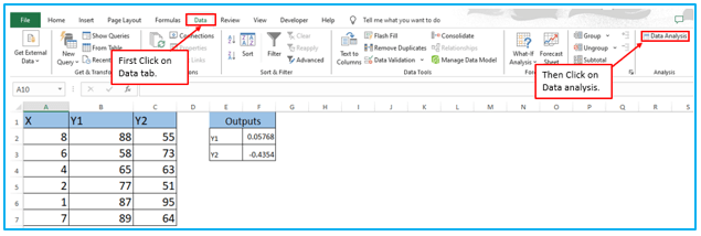
Step 10: After clicking on OK tab now Click on Data ˃Data Analysis.
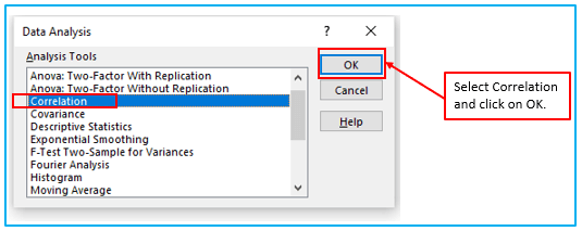
Step 11: After clicking on Data analysis, A dialogue box opens. A dialogue box appears. When getting the dialogue box you can see Correlation from the list of options.
Select Correlation from the list of options and Click OK.
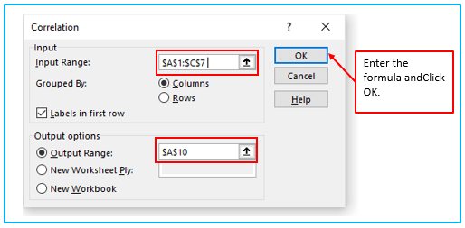
Step 12: After clicking on OK from the above step a Correlation menu will appear like the below image.
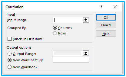
Step 13: In this menu first provide the Input Range. The input range is the cell range of X and Y1 columns and also, supplies the Output Range as the cell number where you want to display the result. As highlighted in the picture below.
Then, Check the Labels in the first-row option if you have labels in the dataset. In this case column 1 has label X and column 2 has label Y1.
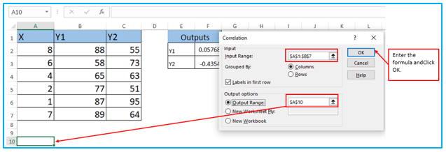
Here entered the range according to the information. For Calculating X and Y1 the formula will be:$A$1:$B$7, Output range $A$10.
When you put the output range you can see a mark there as shown below according to given output range.
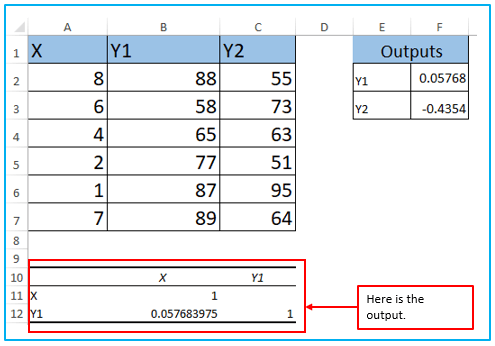
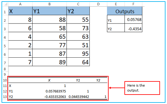
Step 14: While clicking on OK, The Data Analysis table is now ready. Here, you can see the correlation coefficient between X and Y1 in the analysis table.
Like the above way, For calculating the correlation coefficient between X and Y2 in the analysis table use this formula: $A$1:$C$7 and Output range is $A$10.
In the below picture, you can see the formula is entered
Step 15: After pressing OK, you will get the correlation between X and Y2
Here is the result below.
You may be interested:
