Color Scales in Excel offer a powerful visual representation of data, allowing users to quickly interpret trends, patterns, and variations. By applying color gradients to cells based on their values, users can easily identify high and low points in their data sets, making it ideal for data analysis, reporting, and presentation purposes. Whether you’re analyzing sales figures, tracking project progress, or evaluating performance metrics, Color Scales in Excel provide a user-friendly way to visualize data and gain insights at a glance. With customizable color scales and formatting options, users can tailor the visualization to suit their specific needs and preferences. Embracing the use of Color Scales in Excel enhances the effectiveness of your data analysis workflows, enabling you to make informed decisions and communicate insights more effectively.
This Tutorial Covers:
- What are Color Scales in Excel
- How to use Color Scales in Excel
- How to create Custom Color Scales in Excel
- How to show Color Scale without Numbers
- How to Customize the Excel Color Scales
- How to Remove Color Scales in Excel
1. What are Color Scales in Excel?
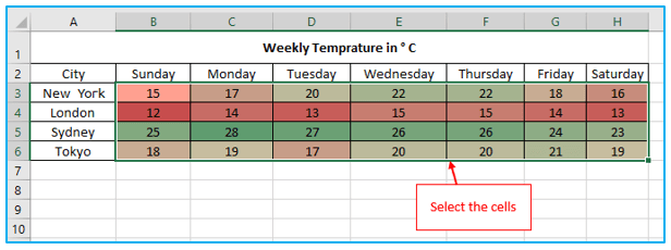
Gradient differentiation within a cell, such as color scales, aids in letting the user know which range the data comes under. The minimum, middle, and maximum points are represented by the corresponding color scales. For instance, using a darker color for a higher value and a lighter hue for a lower value can make it simpler to compare and determine the values.
Color gradations are frequently used to depict earnings, investments, temperature, time, and other measurable elements.
Depending on the data, you can choose between two and three color scales. You can input the data using color scales and conditional formatting, and Excel will highlight the specific cell containing the value depending on the threshold you specify.
2. How to use Color Scales in Excel?
Color scales in Excel allow you to visualize data using different colors based on their values.
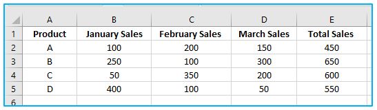
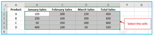
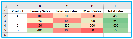
Let’s say you have a sales report for different products over a period of time. The table consists of the following columns: Product, January Sales, February Sales, March Sales, and Total Sales.
Here’s a step-by-step guide to using color scales in Excel:
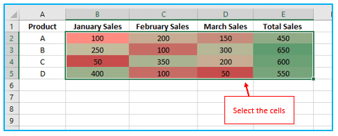
Step 1: Select the range of cells that you want to apply the color scales to. In this case, select the range from B2 to E5 (January Sales to Total Sales).

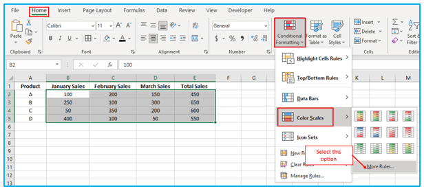
Step 2: Go to the “Home” tab in the Excel ribbon. In the “Styles” group, click on “Conditional Formatting.” From the drop-down menu, select “Color Scales.”
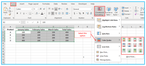
There are 12 preset color schemes available in Excel. There are 12 total, of which 6 are two-color scales and 6 are three-color scales. You may see a preview of the color scales and their descriptions when you hover over them.
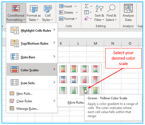
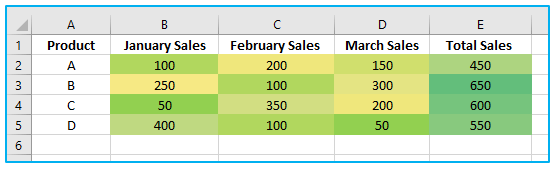
Step 3: The color scales are applied to the chosen data once you click on them. We have chosen the Green-Yellow color scheme in this instance.
Based on the values in each cell, Excel will apply the color scale to the selected range of cells. A darker shade of the selected color will be assigned to cells with higher values, while cells with lower values will receive a lighter shade.
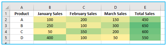
This is a quick and effective technique to apply the color scales to the chosen data so you can quickly grasp it.
Note: The conditional formatting skips any blank cells or values with errors and highlights the other cells when the selected data has either.
3. How to create Custom Color Scales in Excel?
You can establish a Custom Color Scales in Excel if one of the fast rules mentioned above doesn’t completely describe how you want your color scale to function.
The steps to create custom color scales in Excel are described below:
Step 1: Select the range of cells that you want to apply the color scales to. In this case, select the range from B2 to E5 (January Sales to Total Sales).
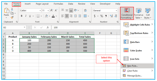
Step 2: Go to the “Home” tab in the Excel ribbon. In the “Styles” group, click on “Conditional Formatting.” From the drop-down menu, select “New Rules”.
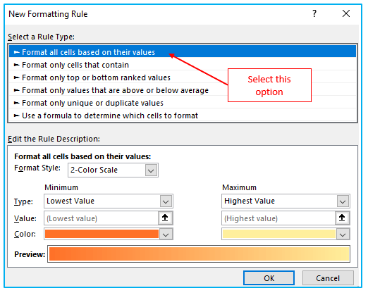
Step 3: Choose “Format All Cells Based on Their Values” in the window that appears after you click “New Formatting Rule” at the top.
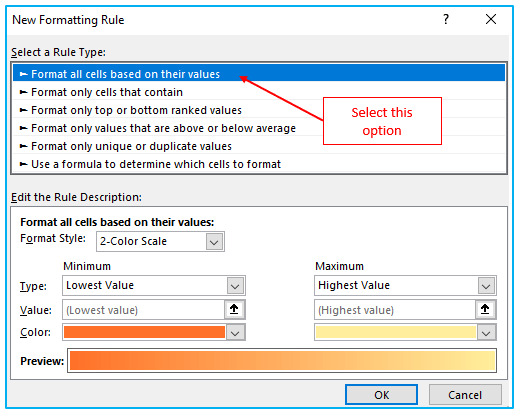
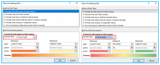
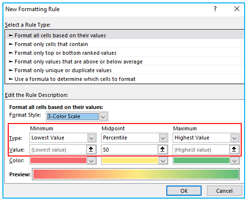
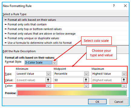
You can customize the rule by spending some time in the “Edit the Rule Description” area at the bottom of the window. Start by selecting “2-Color Scale” or “3-Color Scale” in the “Format Style” drop-down menu for multiple color scales.
The three-color scale has a midway, whereas the two-color scale only contains lowest and maximum values. This is the primary distinction between these two styles.
Step 4: Choose the Minimum, Maximum, and, if desired, the Midpoint using the Types drop-down menus. Lowest/Highest Value, Number, Percent, Formula, or Percentile are the options you have.
You don’t need to enter anything in the Value boxes because the Lowest Value and Highest Value types are based on the information in the range of cells you’ve chosen. Enter the Values in the relevant fields for all other categories, including Midpoint.
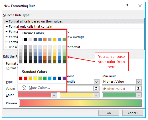
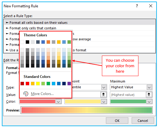
Step 5: Finally, choose your colors from the palettes by clicking the “Color” drop-down buttons. Select “More Colors” to add custom colors using RGB or Hex values if you wish to do so.
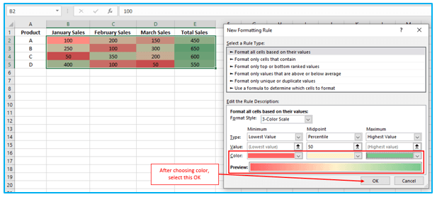
A preview of your color scale will then appear at the bottom of the window. Click “OK” to apply the conditional formatting to your cells if you’re satisfied with the outcome.
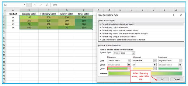
This type of conditional formatting rule has the benefit of automatically updating the color scale to reflect any changes you make to your data.
4. How to show Color Scale without Numbers?
Excel does not offer the Show Scale Only option for color scales the same way it does for icon sets and data bars. However, you may quickly conceal numbers by using a unique custom number format.
To hide the numbers and only display the color scale in Excel, you can follow these steps:
Step 1: Select the range of cells that contain the color scale you want to modify.
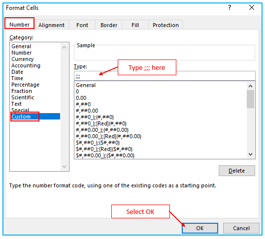
Step 2: Press Ctrl + 1 to open the “Format Cells” dialog box.
In the “Format Cells” dialog box, select the “Number” tab. Select “Custom” from the list of categories. In the “Type” box, delete any existing format code and enter three semicolons (;;;) as the new format code. Click OK to apply the changes.
By using three semicolons as the format code, Excel will hide the numerical values in the selected range and only display the color scale.
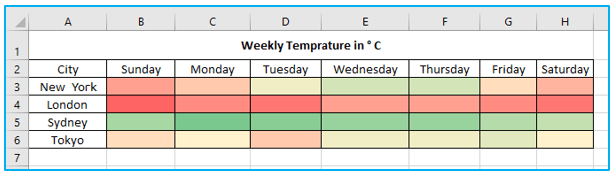
Please note that this method hides the actual values but retains the formatting. If you need to see the values again, you can revert the formatting by selecting the range, opening the “Format Cells” dialog box, and changing the formatting back to the desired option.
5. How to Customize the Excel Color Scales?
You can assign the values from the More Rules section when you need to change the color based on particular values.
The steps to customize the Excel color scales are described below:
Step 1: Select the range of cells that you want to apply the color scales to. In this case, select the range from B2 to E5 (January Sales to Total Sales).

Step 2: Go to the “Home” main menu after that. Select “Conditional Formatting” from the dropdown menu under the “Styles” section. Click “More Rules” in the “Color Scales” section after expanding it.
Step 3: The “New Formatting Rule” dialog box appears after doing this. In this dialog box, choose “Format All Cells Based on Their Values” in the window that appears after you click “New Formatting Rule” at the top.
Step 4: Using the Types drop-down choices, select the Minimum, Maximum, and, if required, the Midpoint. You can choose from Lowest/Highest Value, Number, Percent, Formula, or Percentile.
The Lowest Value and Highest Value kinds are dependent on the data in the cells you’ve selected, so you don’t need to enter anything in the Value boxes. Fill in the values in the appropriate fields for Midpoint and all other categories.
Step 5: Finally, choose your colors from the palettes by clicking the “Color” drop-down buttons. Select “More Colors” to add custom colors using RGB or Hex values if you wish to do so.
A preview of your color scale will then appear at the bottom of the window. Click “OK” to apply the conditional formatting to your cells if you’re satisfied with the outcome.
This type of conditional formatting rule has the benefit of automatically updating the color scale to reflect any changes you make to your data.
6. How to Remove Color Scales in Excel?
Occasionally, you could decide not to include the color scales in the chosen cells after applying the color scales to the data.
If this is the case, you can choose to delete them by following the instructions below:
Step 1: Select the cells that you want to be free of color scales first.
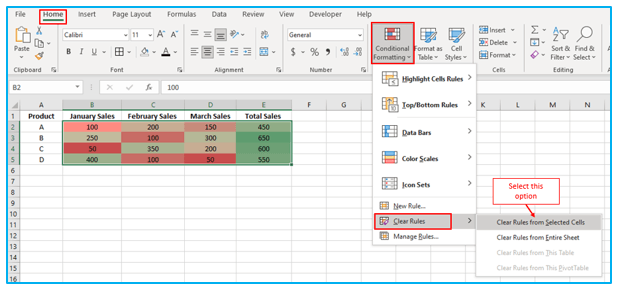
Step 2: Go to the “Home” tab by navigating. Choose “Conditional Formatting” from the drop-down menu, then expand the “Clear Rules” menu options before selecting “Clear Rules from Selected Cells”. Click “Clear Rules from Entire Sheet” to remove the color scales from the entire spreadsheet.
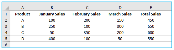
By doing this, the color scaling in the chosen cells is immediately removed.
This tutorial provides practical guidance on using color scales in Excel for effective data visualization. By assigning different colors to values, color scales enable quick identification of patterns and trends. The tutorial includes a real-life example of temperature data for cities over a week to demonstrate the application of color scales. The step-by-step instructions simplify the process of applying color scales in Excel, and a bonus tip explains how to hide numbers, display only the color scale, and remove the color scale. Mastering color scales empowers users to enhance data analysis and communicate insights visually.
Application of Color Scales in Excel
- Data Analysis: Color Scales in Excel visually represent data trends, making it easier to identify patterns and anomalies.
- Performance Evaluation: Users can apply color scales to performance metrics, allowing for quick assessment and comparison of results.
- Financial Reporting: Color-coded gradients in Excel enhance financial reports by highlighting key figures and trends for better comprehension.
- Project Tracking: Color scales aid in tracking project progress by visually indicating task completion levels or milestone achievements.
- Risk Assessment: Users can use color scales to assess risks by highlighting areas of concern or potential issues in data sets.
- Comparative Analysis: Color scales facilitate comparative analysis by visually comparing data sets side by side for better decision-making.
For ready-to-use Dashboard Templates:
