Microsoft Excel offers a wide array of powerful functions to help you manipulate and analyze your data effectively. One such function is CEILING, which is specifically designed to round numbers up to a specified multiple. Whether you’re dealing with financial data, sales figures, or any other numerical values, the CEILING function can be a valuable tool in your Excel arsenal.
In this tutorial, we will walk you through the step-by-step process of using the CEILING function, exploring its syntax, arguments, and practical examples. By the end of this guide, you’ll have a solid understanding of how to leverage the CEILING function to round up numbers and tailor it to your specific needs.
This Tutorial Covers:
- What is the Excel CEILING Function
- Syntax
- Arguments
- How to use the CEILING Function in Excel
- Example 1 – Basic Excel Ceiling
- Example 2 – Using CEILING with other functions
- CEILING Tips & Tricks
- Common mistakes when using CEILING
- Why isn’t CEILING Function working
- CEILING: Related Formulae
1. What is the Excel CEILING Function?
The Excel CEILING function is categorized under the “Math and Trigonometry” functions in Microsoft Excel. Its primary purpose is to round a given number up to the nearest multiple of a specified number, regardless of whether the number is positive or negative.
This function is particularly valuable in financial analysis and modeling. For instance, when dealing with currency conversions or calculating discounts, CEILING can be used to ensure that prices are set appropriately and align with specific increments. In financial models, CEILING enables rounding up numbers as per the necessary requirements, ensuring accuracy and precision in calculations.
By using the CEILING function effectively, you can streamline your financial calculations and ensure that your data conforms to predetermined rules or standards. This makes it a versatile tool for various applications, where precision and consistency are essential.
- Syntax:
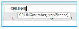
Following is the syntax for Excel’s CEILING function:
=CEILING(number, significance)
- Arguments:
Following is the arguments for Excel’s CEILING function:
number (required argument): This is the value that you want to round off to the nearest multiple. It can be a cell reference containing the number, a constant value, or a formula that evaluates to a number.
significance (required argument): This is the multiple or step value to which you want to round up the number. The CEILING function will round the number up to the nearest multiple of this value, maintaining the same arithmetic sign (positive or negative) as the provided number argument.
2. How to use the CEILING Function in Excel?
Let’s examine some instances to better understand the real-world uses for the Excel CEILING formula in the next section of this tutorial.
- Example 1 – Basic Excel Ceiling:
Suppose we have a dataset representing like below.
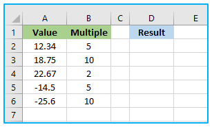
In this example, we have a dataset in columns A and B. Column A contains various values, and column B represents the multiples to which we want to round up these values using the CEILING function.
Column D is where we apply the CEILING function to round the numbers in column A up to the nearest multiple specified in column B.
The steps to use CEILING formula in Excel are described below:
Step 1: Apply the below formula in cell D2 and you can either copy and paste the formula or drag the formula’s fill handle to the remaining cells.
=CEILING(A2,B2)
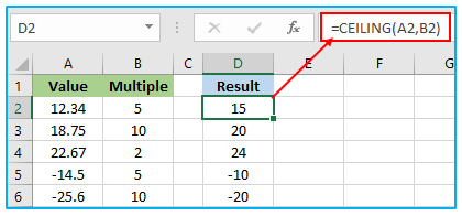
In cell D2, this formula rounds the value 12.34 up to the nearest multiple of 5, resulting in 15. Similarly, all remaining cell’s value is rounded up.
The CEILING function is applied to each corresponding pair of values from columns A and B, allowing us to round the numbers up to the specified multiples and generate the results in column C. This is just one basic example of how the CEILING function can be used in Excel for rounding up numbers as per specific requirements.
- Example 2 – Using CEILING with other functions:
In this example we’ll use the Excel CEILING function along with the AVERAGE function to round up the average rating of a product or service and display it as a whole number.
Suppose we have the following dataset:
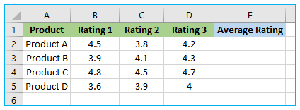
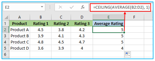
In this example, we have a list of products in column A. Columns B, C, and D represent the individual ratings for each product. Column E displays the average rating of each product.
To calculate the average rating and ensure it is displayed as a whole number, we’ll use the CEILING function along with the AVERAGE function.
The steps to use CEILING with other function in Excel are described below:
Step 1: Apply the below formula in cell E2 and you can either copy and paste the formula or drag the formula’s fill handle to the remaining cells.
=CEILING(AVERAGE(B2:D2), 1)
Here’s how the formula works:
AVERAGE(B2:D2): This calculates the average rating of Product A by taking the average of the ratings in cells B2, C2, and D2. For example, (4.5 + 3.8 + 4.2) / 3 = 4.5.
CEILING(AVERAGE(B2:D2), 1): The CEILING function then rounds up this average rating to the nearest whole number. In this case, CEILING(4.5, 1) gives us 5.
The formula is similarly applied to other rows in column E, using the corresponding values from columns B, C, and D.
By using the CEILING function together with the AVERAGE function, we can ensure that the average rating of each product is rounded up to a whole number, providing a clear and concise representation of customer satisfaction.
3. CEILING Tips & Tricks
Here are some helpful tips and tricks to maximize the utility of the CEILING function in Excel:
- Even if the value is already a multiple of the specified significance, the CEILING function always rounds up. Instead, you might want to use the FLOOR function if you need to round down.
- Use the CEILING function with a significance of 1 to round an integer to the nearest whole number.
- The CEILING function can be used to round up time values to the nearest hour, minute, or second. Just enter the proper significance value—for example, 1/24 for hours, 1/1440 for minutes, or 1/86400 for seconds—in the appropriate field.
These pointers and techniques will help you get the most out of Excel’s CEILING function and speed up your data handling and calculations.
4. Common mistakes when using CEILING
Here are some common mistakes to be mindful of when using the CEILING function in Excel:
- Forgetting to include both the number and significance arguments in the function will lead to an error. Always ensure that you provide both arguments to the CEILING function for it to work correctly.
- working with positive integers and applying a negative value for the significance argument, or the opposite. This will also result in an error. Make sure the significance value aligns with the sign of the number you are rounding.
- Neglecting to consider the impact of rounding up on your calculations, particularly when dealing with large data sets or financial figures. Always verify your results to ensure they accurately reflect the rounded values.
By being aware of these potential pitfalls, you can avoid errors and make effective use of the CEILING function to round numbers up efficiently and accurately in your Excel spreadsheets.
5. Why isn’t CEILING Function working?
If you encounter difficulties with the CEILING function in Excel, keep the following troubleshooting tips in mind:
- Make sure to include both the number and significance arguments in the function. Without both arguments, the CEILING function will not produce the desired result.
- Check that the significance argument has the appropriate sign (positive or negative) based on the number you’re rounding. Using the wrong sign may lead to incorrect rounding.
- Verify that your formula is entered accurately, without any typographical errors or syntax mistakes. Even a small error can prevent the function from working correctly.
- Consider any formatting issues that may affect the display of your results. Check the number formatting and cell formatting to ensure they align with your expected output.
By being mindful of these troubleshooting tips, you can effectively use the CEILING function and resolve any potential issues that arise while working with it in Excel.
6. CEILING: Related Formulae
Here are some related formulae that complement the CEILING function in Excel, providing you with a broader set of rounding and truncating options:
- FLOOR: This function rounds a number down to the nearest multiple of a specified value. Its syntax is similar to the CEILING function: `=FLOOR(number, significance)`.
- ROUND: With this function, you can choose how many decimal places to round a number to. The syntax is `=ROUND(number, num_digits)`, where `num_digits` indicates the number of decimal places to round to.
- MROUND: This function rounds a number to the nearest multiple of a specified value, either up or down depending on the number. The syntax is `=MROUND(number, multiple)`.
- INT: This function rounds a number down to the nearest integer. The syntax is `=INT(number)`.
- TRUNC: This function truncates a number to a specified number of decimal places, effectively removing any decimal portion beyond the specified number of places. The syntax is `=TRUNC(number, [num_digits])`, where `num_digits` is an optional argument that defaults to 0 if not provided.
By understanding and utilizing these related formulae in conjunction with the CEILING function, you can round and truncate numbers in various ways, making your calculations more precise and adaptable to different scenarios. With this comprehensive knowledge, you should now be well-equipped to master the CEILING function and its related formulae in Excel.
You may be interested:
