Automatic formatting in Excel is a transformative feature that brings efficiency and visual appeal to your spreadsheets. It’s essential for anyone looking to present data in a clear, consistent, and visually appealing manner. Whether you’re a financial analyst illustrating complex data sets, a marketer tracking campaign metrics, or an educator organizing student information, mastering automatic formatting can significantly enhance your productivity. This guide will walk you through the ins and outs of using automatic formatting in Excel, empowering you to transform your raw data into professionally styled spreadsheets with just a few clicks, ensuring that your information is not only accurately represented but also aesthetically pleasing.
Potential uses for automatic formatting in Excel
- Highlighting cells that meet certain conditions, such as those that contain values above or below a certain threshold.
- Creating a color-coded heat map to quickly visualize trends in your data
- Applying formatting to cells based on the data type, such as making all dates display in a specific format
- Automatically format cells based on data that is entered or updated, so your spreadsheet always looks consistent and organized
This Tutorial Covers:
- Where is Excel’s AutoFormat or Automatic Formatting?
- Data Auto Formatting Using the AutoFormat Option
- Changing the AutoFormat formatting design
- Removing the automatic formatting from the dataset
- Limitations of Excel’s AutoFormat option
1. Where is Excel’s AutoFormat?
If the AutoFormat option is not there in Excel’s ribbon or Quick Access Toolbar, then you won’t be able to access it there (QAT).
It must be manually added to the QAT.
The steps to include the AutoFormat option in the QAT are as follows:
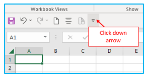
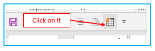
Step 1: First, go to your quick access toolbar and select the little down arrow at the toolbar’s endpoint.
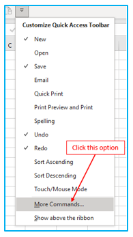
Step 2: Additionally, a drop-down menu will appear when you click on it. Select “More Commands” from this menu.
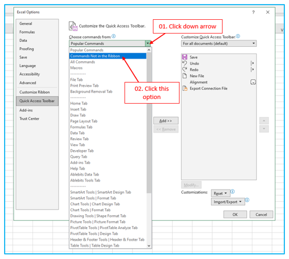
Step 3: When you click on it, Excel’s settings will pop up to let you “Customize the Quick Access Toolbar.”
Choose “Commands Not in the Ribbon” from the “Choose commands from” drop-down menu by clicking here.
Step 4: Then proceed to the list of commands that is immediately below this drop-down.
Add the “Auto Format” option to the fast access toolbar after choosing it and then select OK.
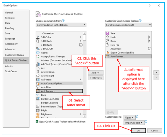
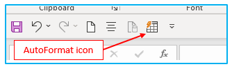
In your fast access toolbar, you now have the auto-format icon.
2. Data Automatic Formatting Using the AutoFormat Option
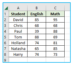
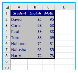
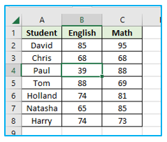
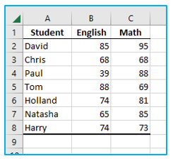
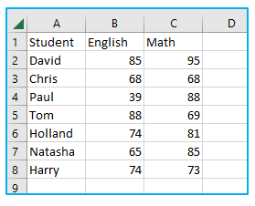
It’s really easy to apply formats when using an auto-format option. Say you wish to format the data table below:
Procedure of data auto formatting using AutoFormat option:
Step 1: Choose any cell in your data by clicking on it.
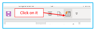
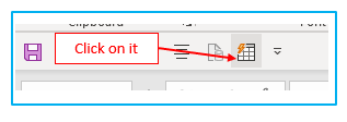
Step 2: Navigate to the quick access toolbar and select the auto-format button.
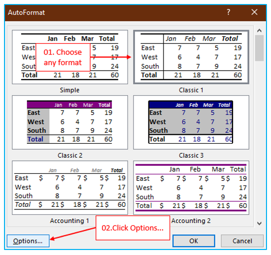
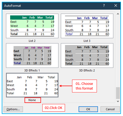
Step 3: You now have a window with a variety of data formats. Click OK after choosing one of them.
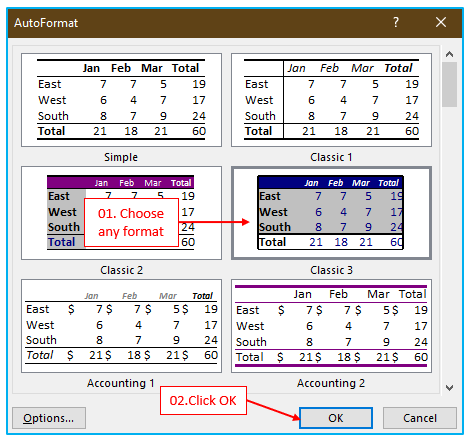
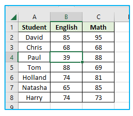
The data will immediately use your selected format after you click OK.
Keep in mind that after using the AutoFormat design, you can adjust the formatting. For instance, you can change the headers’ color to any other color if you don’t like it.
Additionally, any formatting that has already been done to the dataset will be overridden. For instance, if you have red header cells and choose a format with a blue header, the blue color will be applied to the cells instead of the red headers.
3. Changing the AutoFormat formatting design
When using the AutoFormat options, you can make a few restricted changes to the formatting layout.
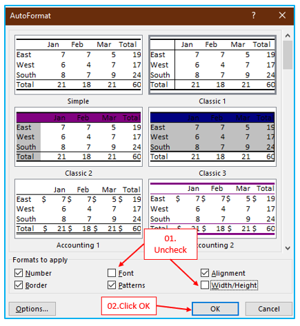
When using AutoFormat, you can enable or disable the following six categories of formats:
- Number Formatting
- Border
- Font
- Patterns
- Alignment
- Width/Height
Let’s imagine you want to format the data table below, but you don’t want to alter the font style or column width.
Changing AutoFormat formatting design by following the instructions below:
Step 1: Choose any cell in your data by clicking on it.
Step 2: Navigate to the quick access toolbar and select the auto-format button.
Step 3: Click the “Options…” button after choosing the format you want to use.
Step 4: Uncheck “Font” and “Width/Height” in the settings menu. Finally, click OK.
Currently, neither of the components is present in your formatting.
4. Removing the automatic formatting from the dataset
The best method for removing formatting from data is to utilize the shortcut key Alt + H + E + F. However, you can easily eliminate formatting from your data by using the auto format option.
The procedure of Removing the formatting from the dataset:
Step 1: Choose any cell in your data by clicking on it.
Step 2: Navigate to the quick access toolbar and select the auto-format button.
Step 3: Go to the “None” format which is the last in the list of formats. Click OK after selecting it.
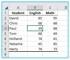
After selecting it, all format will be removed. The result looks like below.
5. Limitations of Excel’s AutoFormat option
This feature has been there for a while, but its usefulness has decreased since Excel’s ribbon introduced more advanced formatting and design options for tables.
Only when your data has a specific structure should you use it, in my opinion (has headers rows, and columns). I advise using separate formatting choices if your data is not organized in this manner.
Additionally, AutoFormat does not allow you to change a single formatting option. For instance, you are unable to make the border thick or dashed.
For ready-to-use Dashboard Templates:
