ABS Function in Excel simplifies numerical analysis by providing a straightforward solution for obtaining absolute values of numbers. Whether you’re dealing with financial data, mathematical calculations, or scientific measurements, ABS Function in Excel ensures accuracy and consistency in your results. Say goodbye to complex formulas or manual calculations and hello to efficiency with this versatile function. From identifying deviations in datasets to ensuring data integrity in formulas, ABS Function in Excel streamlines your workflow, saving you time and effort. Take control of your numerical analysis tasks and optimize your Excel experience with the powerful capabilities of ABS Function. With just a simple formula, you can easily obtain absolute values, making it easier to interpret and utilize your data effectively. Embrace the convenience and reliability of ABS Function in Excel and elevate your spreadsheet skills to new heights of productivity and accuracy.
This Tutorial Covers:
- What is the ABSOLUTE Function in Excel (ABS)?
- Syntax
- Arguments
- Usage notes
- How to calculate the absolute value in Excel
- Convert negative numbers to positive numbers
- Find if the value is within the tolerance
- How to sum absolute values in Excel
- How to determine the maximum/minimum absolute value
- How to do average absolute values in Excel
- More absolute value formula examples
1. What is the ABSOLUTE Function in Excel (ABS)?
Excel’s ABS Function provides a number’s absolute value. Positive numbers are unchanged while negative numbers are converted to positive numbers by the function.
-
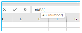
Syntax:
The syntax of the ABS function in Excel is as follows:
ABS(number)
-
Arguments:
The arguments of the ABS function in Excel is as follows:
number – Here, “number” is the numeric value for which you want to find the absolute value.
-
Usage notes:
The ABS function in mathematics returns the distance of a number from zero on a number line. In computing, the ABS function returns the absolute value of a number. The absolute value of a number is the number itself if it’s positive or zero, and the negative of the number if it’s negative.
The ABS formula in Excel takes only one argument, which is the number whose absolute value you want to find. It must be a numeric value; otherwise, the function returns a #VALUE! error.
2. How to calculate absolute value in Excel?
Now that you are familiar with the idea of absolute value, let’s look at some practical uses for the Excel ABS formula. The following examples will help you comprehend what absolute value is and how it can be applied in different situations.
3. Convert negative numbers to positive numbers:
The Excel ABS function is a simple option when you need to convert negative numbers to positive numbers.
Let’s say that you subtract two lengths to find their difference. The issue is that while you want the difference to always be a positive number, some of the outputs are negative numbers:
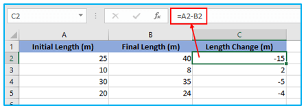
How to convert negative numbers to positive numbers is shown below:
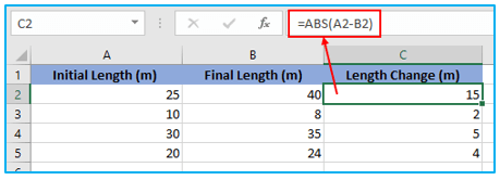
Step 1: Put the following formula inside the ABS function:
=ABS(A2-B2)
and make the positive numbers unchanged while the negative numbers are changed from negative to positive:
-
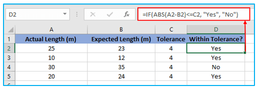
Find if value is within tolerance:
Finding out whether a given value (number or percentage) is within expected tolerance or not is another typical use of Excel ABS function.
You construct the formula as follows using the actual value in A2, the expected value in B2, and the tolerance in C2:
- Get the absolute value of the difference by deducting the predicted value from the actual value (or the other way around): ABS(A2-B2)
- Verify that the absolute value is less or equal to the tolerance allowed: ABS(A2-B2)<=C2
- Return the desired messages by using the IF statement. In this example, if the difference is within tolerance, we return “Yes,” otherwise “No”
=IF(ABS(A2-B2)<=C2, “Yes”, “No”)
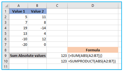
4. How to do sum absolute values in Excel?
Use one of the following formulas to obtain the total value of all the numbers in a range:
Array formula:
SUM(ABS(range))
Regular formula:
SUMPRODUCT(ABS(range))
In the first instance, you instruct the SUM function to sum up every number in the given range by using an array formula. SUMPRODUCT can handle a range without the need for additional processing because it is an array type function by nature.
Either of the formulas listed below will work great with the numbers to be added in cells A2 through B7:
- Ctrl + Shift + Enter is used to finish the following array formula:
=SUM(ABS(A2:B7))
- Typical Enter keystroke is used to finish the following regular formula:
=SUMPRODUCT(ABS(A2:B7))
The two formulas ignore the sign and add the absolute values of positive and negative numbers, as seen in the screenshot below:
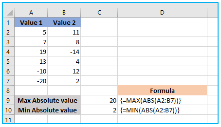
5. How to determine the maximum/minimum absolute value?
Using the following array formulae is the simplest technique to find Excel’s minimum and maximum absolute values.
Maximum absolute value:
MAX(ABS(range))
Minimum absolute value:
MIN(ABS(range))
The formulas have the following form when applied to our sample dataset in A2:B7:
- To obtain the maximum absolute value:
=MAX(ABS(A2:B7))
- To determine the minimum absolute value:
=MIN(ABS(A2:B7))
By hitting Ctrl+Shift+Enter, please make sure the array formulae are completed correctly.
If you prefer not to use array formulae in your worksheets, you can force the ABS function to process a range by nesting it inside the INDEX function’s array parameter as seen in the example below.
To obtain the maximum absolute value:
=MAX(INDEX(ABS(A2:B7),0,0))
To determine the minimum absolute value:
=MIN(INDEX(ABS(A2:B7),0,0))
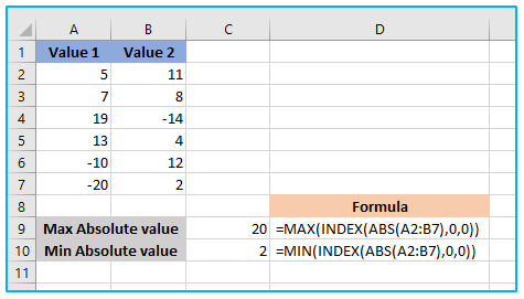
This works because Excel is instructed to return an entire array rather than a single result by an INDEX formula with the row_num and column_num parameters set to 0 or omitted.
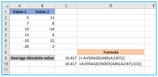
6. How to do average absolute values in Excel?
The same formulas we used to determine the minimum and maximum absolute value are also capable of averaging absolute values. All you have to do is swap out MAX/MIN for the AVERAGE function:
Array formula:
=MAX(ABS(range))
Regular formula:
=AVERAGE(INDEX(ABS(range),0,0))
The following are the formulas that might apply to our sample data set:
- Input the following array formula in cell C9 by pressing Ctrl + Shift + Enter:
= AVERAGE(ABS(A2:B7))
- Regular formula for averaging absolute values:
=AVERAGE(INDEX(ABS(A2:B7),0,0))
7. More absolute value formula examples:
In addition to its typical uses, the ABS function in Excel can be combined with other functions to handle tasks that don’t have built-in solutions. Here are a few examples:
- Getting the date closest to today: Use the ABS function to find the difference between today’s date and a list of dates, and then use the MIN function to find the date with the smallest absolute value difference.
- Ranking numbers by their absolute values: Use the RANK function with an array formula that utilizes the ABS function to rank numbers based on their absolute values, ignoring the sign.
- Extracting the decimal part of a number: Use the ABS function with the TRUNC function to remove the integer part of a number and return the fractional part as an absolute value.
- Taking the square root of a negative number: Get the square root of a negative number as if it were positive by using the SQRT function after using the ABS function to get the absolute value of the negative number.
That is how to use Excel’s ABS function to calculate an absolute number. The formulas covered in this tutorial are extremely simple, so it won’t be difficult for you to adapt them for your worksheets.
Application of ABS Function in Excel
- Absolute Values: Calculate the absolute value of numbers, disregarding their sign, using the ABS function in Excel.
- Error Handling: Use ABS to convert negative numbers to positive values, facilitating error handling in formulas or calculations.
- Distance Calculations: Determine distances or differences between values by obtaining their absolute values with the ABS function.
- Trend Analysis: Analyze trends or patterns in data by obtaining the absolute values of deviations from a baseline using ABS.
- Financial Modeling: Apply ABS to financial models to ensure accurate representation of cash flows, returns, or asset values.
- Data Normalization: Normalize data by converting negative values to positive counterparts with the ABS function, facilitating comparative analysis and visualization.
For ready-to-use Dashboard Templates:
