Strikethrough text in Excel offers a versatile way to visually indicate changes, completed tasks, or canceled items within your spreadsheet. By applying strikethrough formatting, you can quickly draw attention to updated information or mark items as completed, making it easier to track progress or identify changes. Whether you’re managing tasks, editing text, or highlighting revisions, utilizing strikethrough text in Excel enhances clarity and organization. With this simple formatting tool, you can streamline your data presentation and improve readability in your Excel documents.
What is Strikethrough?
A strikethrough is plainly a line that runs through the middle of a word. It is indeed ideal for working together and showing others which words you believe should be eliminated.
How to add a strikethrough in Excel through a keyboard shortcut?
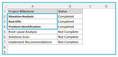
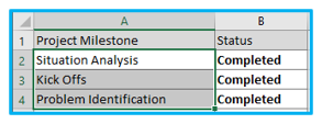
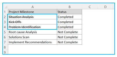
Step 1: Select the cells to do the strikethrough, here we select cells A2:A4 the project milestones that status is completed.
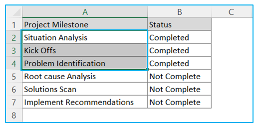
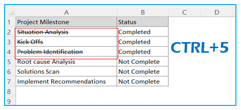
Step 2: Now press CTRL+5 to strikethrough the selected cells.
How to add a strikethrough in Excel through Format Cell Option?
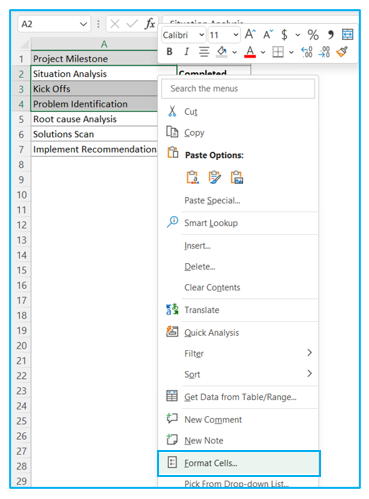
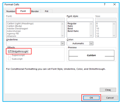
Step 1: Select the cells to do the strikethrough, here we select cells A2:A4 the project milestones that status is completed. Right-click and select ‘Format Cells’ as indicated in the image.
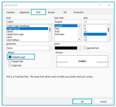
Step 2: From the following Format Cells window select Font, Effects as Strikethrough, and hit OK
You can derive this Format Cells window by pressing CTRL+1.
Step 3: After clicking OK, your selected text will be in Strikethrough format. Results outlined below:
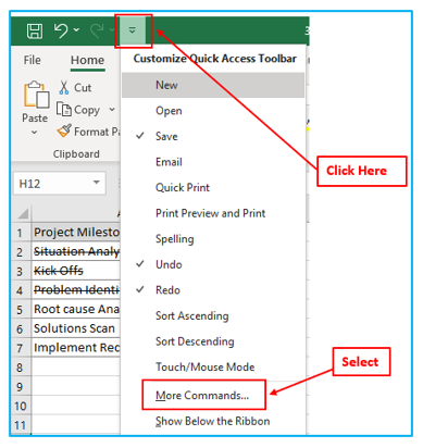
How to add a strikethrough button to Quick Access Toolbar?
Step 1: Select More commands from the drop-down menu by clicking the down arrow to the right of the Quick Access Toolbar. The Options window appears.
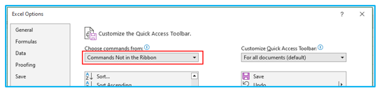
Step 2: Select “Commands Not in the Ribbon” from the “Choose commands from” menu.
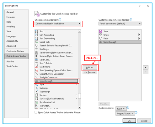
Step 3: Click Strikethrough in the list of commands, then click Add.
Step 4: Select OK. The strikethrough icon will now appear in the quick access toolbar.
Step 5: Select the cells to do the strikethrough.
Step 6: Click on the “Strikethrough button”. It will strikethrough the selected cells.
How to strikethrough automatically with conditional formatting?
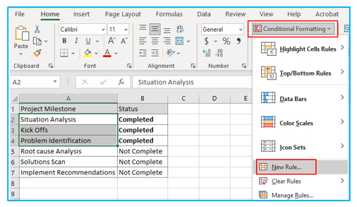
Step 1: Select the cells to do the strikethrough, here we select cell A2:A4 the project milestones.
Step 2: Select “Conditional Formatting,” and then “New Rule.”
Step 3: Simply tap on “Use a formula to determine which cells to format,” then enter the formula (=B2=” Completed”) and press “Format.”
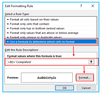
Step 4: Select the Strikethrough option in the Font tab from the Format Cells dialog box.
Step 5: Click OK. It would implement the strikethrough format to the selected cells.
Application of Strikethrough Text in Excel
- Indicate completed tasks: Use strikethrough text to mark tasks as completed.
- Highlight changes: Cross out old information to indicate updates or revisions.
- Remove duplicates: Strike through duplicate entries to identify and remove them easily.
- Track progress: Strikethrough text can show progress made or items that no longer apply.
- Show cancelled items: Use strikethrough to indicate cancelled appointments, orders, or events.
- Edit text: Cross out incorrect or unnecessary text before making revisions.
For ready-to-use Dashboard Templates:
