Shade or Color Alternate Rows in Excel is a simple yet effective technique to improve the readability and visual appeal of your spreadsheets. By applying alternating shades or colors to rows, you can make it easier for users to distinguish between different sets of data, reducing eye strain and enhancing comprehension. Whether you’re creating financial reports, tracking inventory, or organizing schedules, implementing Shade or Color Alternate Rows in Excel can elevate the professionalism and clarity of your documents. With just a few clicks, you can transform a bland spreadsheet into a polished and professional-looking document that impresses stakeholders and facilitates better decision-making. Harness the power of Shade or Color Alternate Rows in Excel to make your data stand out and leave a lasting impression.
This Tutorial Covers:
- Alternating row shade or color in Excel
- Shade or color every other row in Excel using banded rows
- How to choose your own colors or shades of row stripes
- How to shade or color a different number of rows in each zebra line
- With one click, remove the alternate rows coloring from Excel
- Alternate row shading using Excel conditional formatting
- Shade or color every other row in Excel using conditional formatting
- How to alternate groups of rows with different colors or shades
- How to shade rows with 3 different colors
- How to alternate row colors or shades based on a value change
- Shade or color every other row in Excel using banded rows
1. Alternating row shade or color in Excel:
Most experts would suggest conditional formatting when asked how to shade or color every other row in Excel, but you’ll need to spend some time learning how to use the MOD and ROW functions in a clever way.
Consider using the built-in Excel table styles as a quick substitute if you’d like not to use a sledgehammer to crack nuts, that is, if you don’t want to waste your time and ingenuity on such a trifle as zebra striping Excel tables.
-
Shade or color every other row in Excel using banded rows:
Utilizing predefined table styles is the quickest and simplest approach to apply Excel row color or shade. Tables have a number of advantages, including automatic filtering and color banding, which is applied to rows by default.
How to shade or color every other row in excel using banded rows is shown below:
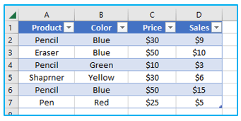
Step 1: Simply converting a set of cells to a table is all that is required. Simply choose your desired range of cells and press “Ctrl+T” at the same time.
When you do this, your table’s odd and even rows will automatically be tinted with distinct colors. The best part is that if you sort, remove, or add new rows to your table, automatic banding will continue.
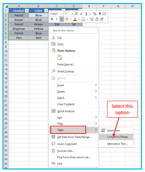
Step 2: You may easily change the table back to a regular range if you’d prefer alternate row shading only, without the table capabilities. Pick any cell in your table, perform a right-click, and then select “Convert to Range” from the context menu to accomplish this.
The final result looks like below:
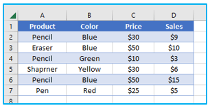
Please take note that the automatic color banding for freshly added rows won’t appear after doing the table-to-range translation. Another drawback of sorting the data is that it distorts the attractive zebra stripe pattern because the color bands follow the original rows.
As you can see, Excel allows you to identify alternative rows quickly and easily by converting a range to a table.
-
How to choose your own colors or shades of row stripes?
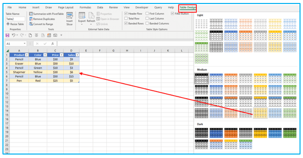
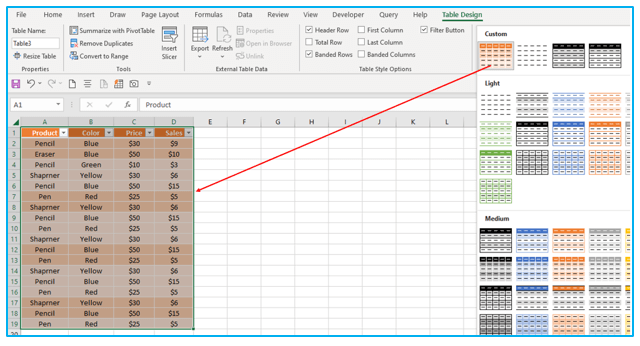
There are many other patterns and colors available if the usual blue and white design of an Excel table does not suit you. Simply choose your table or any cell inside it, go to the “Table Design” tab and select “Table Styles” group, and pick your preferred color scheme.
To examine all of the various table styles, click the More button or use the arrow buttons to go through them. Any style that you hover your mouse over will instantly reflect in your table so you can see how your banded rows will appear.
-
How to shade or color a different number of rows in each zebra line?
You will need to develop a unique table style if you want to draw attention to a particular number of rows in each stripe, such as shading two rows in one color and three in another. Perform the subsequent actions after converting a range to a table, assuming you have already done so.
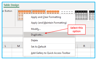
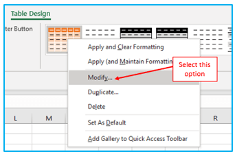
Step 1: Choose “Duplicate” from the context menu when you right-click the table style you want to use in the “Table Design” tab.
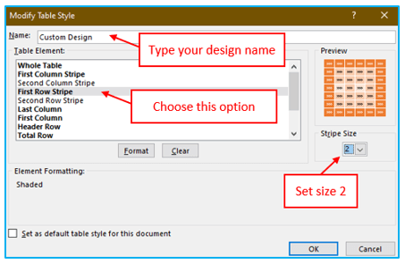
Step 2: Enter the name of your table style in the Name box. Choose “First Row Stripe” and change the Stripe Size to 2 or another number of your choosing.
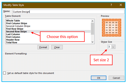
Step 3: Repeat the process by selecting “Second row stripe”. To save your personalized style, click OK.
Step 4: By choosing it from the Table Styles collection, you may apply the newly created style to your table. Your own styles are always accessible in the Custom section at the top of the gallery.
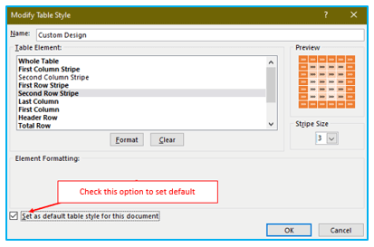
The current workbook is the only place that custom table styles are kept, therefore your other workbooks cannot access them. Select the “Set as default table style for this document” check box when creating or updating the style to make your custom table style the default table style in the current worksheet.
When you right-click your custom style in the Styles Gallery and select “Modify…” from the context menu, you may simply change it if you’re not satisfied with it.
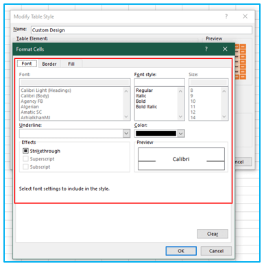
You have lots of room to express your creativity here! As shown in the screenshot below, you can set any Font, Border, and Fill styles as well as select gradient stripe colors on the respective tabs. You can find these options by selecting the “Format” button in the “Modify Table Style” dialog box, and a new dialog box named “Format Cells” will open.
-
With one click, remove the alternate rows coloring from Excel:
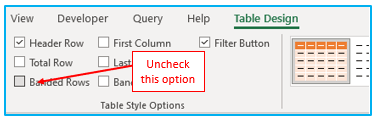
Color banding in Excel tables can be removed with a single click if you want to clear row color or shade in Excel. Go to the “Table Design” tab, select any cell in your table, and uncheck the box for “Banded Rows”.
As you can see, Excel’s built-in table styles offer a multitude of options for changing the color of your worksheet rows and making unique banded row designs. You’ll need to use conditional formatting if you want something unusual, like coloring rows or entire rows based on a change in value.
-
Alternate row shading using Excel conditional formatting:
Of course, conditional formatting is more difficult than the Excel table styles we just covered. But it does have one undeniable advantage: it gives you more creative freedom to zebra stripe your worksheet anyway you see suitable for each unique situation. You can find a few examples of Excel formulas for alternating row colors further on in this article:
- Shade every other row
- Shade groups of rows with different colors
- Shade or color rows using 3 colors
- Alternate rows based on value change
-
Shade or color every other row in Excel using conditional formatting:
Beginning with a very basic MOD formula that shade or colors every other row in Excel, let’s go on. In reality, you can accomplish the same thing using Excel Table styles, but the key advantage of conditional formatting is that it also works for ranges. While a result, your color banding will stay in place as you sort, insert, or delete rows in a range of data to which your formula applies.
This is how a conditional formatting rule is made:
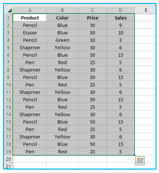
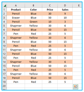
Step 1: Choose the cells you want to shade.
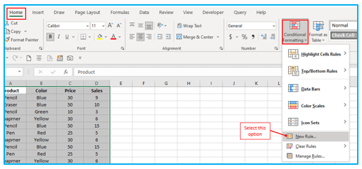
Step 2: Select the Conditional Formatting > New Rule option under the Styles category in the “Home” menu.
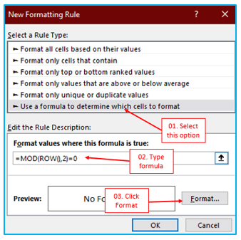
Step 3: Select “Use formula to select which cells to format” in the New Formatting Rule window, then type the following formula: =MOD(ROW() ,2)=0
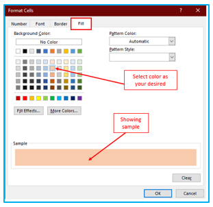
Step 4: Then select the background color you wish to use for the banded rows by clicking the “Format” button, switching to the “Fill” tab.
The chosen color will now be displayed under Sample. Click OK if you’re satisfied with the color.
Step 5: You can click OK once more to apply the color to each additional row in the selected rows after you return to the “New Formatting Rule” window.
And the end result is shown here.
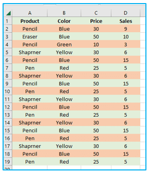
Instead of utilizing white lines, you can build a second rule using this formula if you’d prefer to use two different colors:
=MOD(ROW(),2)=1
The odd and even rows are now marked in distinct colors:
Wasn’t it very simple? In order to use the MOD function in future, slightly more complicated examples, I’d like to quickly go through its syntax today.
After the number has been divided by the divisor, the MOD function provides the remainder rounded to the nearest integer.
For instance, =MOD(4,2) gives 0 because 4 and 2 are equally divisible by 2. (Without remainder).
Let’s examine the MOD function we used in the example above in more detail. As you may recall, we combined the ROW and MOD functions: =MOD(ROW(),2) The ROW method produces the row number, while the MOD function divides it by 2 and provides the result, which is then rounded to the nearest integer. The formula produces the following outcomes when used on our table:
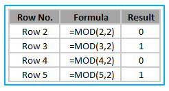
Recognize the trend? For even rows, it is always 0 while for odd rows, it is 1. Then, we develop the conditional formatting rules that instruct Excel to shade or color odd rows (where the MOD function returns 1) in one color and even rows (where the MOD function returns 0) in another.
Let’s look at some more complex instances now that you are familiar with the fundamentals.
-
How to alternate groups of rows with different colors or shades?
Regardless of the information they contain, you can shade or color a certain number of rows using the following formulas:
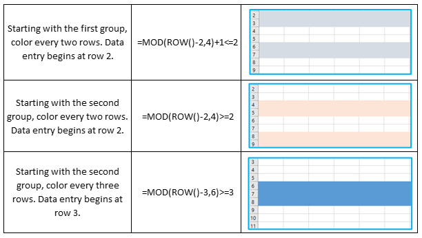
Odd row shading, or emphasizing the first group and each subsequent group:
=MOD(ROW()-RowNum,N*2)+1<=N
To shade or color the second group and all even groupings, use even row shading:
=MOD(ROW()-RowNum,N*2)>=N
Where N is the number of rows in each banded group and RowNum is a reference to the first cell that contains data.
Tip: Use both of the formulas above to construct two conditional formatting rules to shade or color both even and odd groupings.
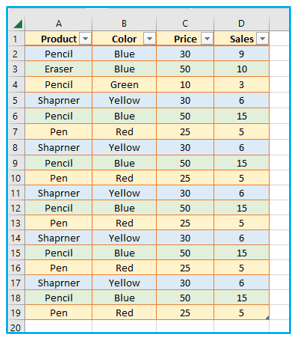
The following table contains a few examples of formula usage and the resulting color banding.
-
How to shade rows with 3 different colors?
If you believe that your data will look better with the rows shaded in three distinct colors, then use the following formulas to construct three conditional formatting rules:
To shade or color 1st and every 3rd row =MOD(ROW($A2)+3-1,3)=1
To shade or color 2nd, 6th, 9th etc. =MOD(ROW($A2)+3-1,3)=2
To shade or color 3rd, 7th, 10th etc. =MOD(ROW($A2)+3-1,3)=0
Keep in mind to replace A2 with a reference to the data-containing first cell.
In your Excel, the resulting table will resemble this:
-
How to alternate row colors or shades based on a value change?
Similar to the assignment we just covered, this one involves darkening groups of rows, but there may be varying numbers of rows in each group.
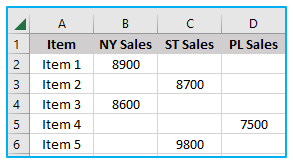
Consider that you have a table with information from many sources, such as regional sales statistics. The first group of rows associated with the first item should be shaded in Color 1, followed by the group associated with the second product in Color 2, and so on. The important column or distinctive identification could be column A, which lists the product names.
You would need a somewhat more complicated algorithm and an additional column to alternate row shading based on change of value:
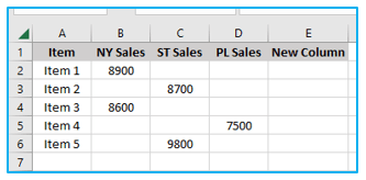
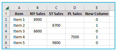
Step 1: Create a new column, say column E, and place it over the worksheet’s right side. Later, you’ll be able to hide this column.
Step 2: If row 2 is your first row with data, enter the following formula in cell E2 and copy it throughout the full column:
=MOD(IF(ROW()=2,0,IF(A2=A1,E1, E1+1)), 2)
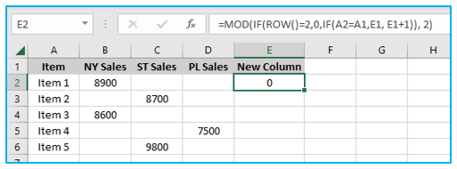
Step 3: Column E will be filled down by blocks of 0 and 1 starting with the item name change, as determined by the formula.
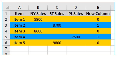
Step 4: Finally, use the formula =$E2=1 to establish a conditional formatting rule. If you want a different color to alternate between blocks of rows, you may add a second rule =$E2=0, as seen in the screenshot:
Application of Shade or Color Alternate Rows in Excel
- Enhanced Readability: Apply alternating shades or colors to rows in Excel to improve readability, making it easier for users to scan and interpret data.
- Data Grouping: Use shading to visually group related data together, helping users quickly identify and understand the structure of your spreadsheet.
- Focus Attention: Highlight important information by shading specific rows, drawing attention to key data points or trends within your dataset.
- Reduced Errors: By making it easier to distinguish between rows, shading can help reduce data entry errors and improve the accuracy of your spreadsheets.
- Professional Presentation: Applying alternate row shading adds a professional touch to your Excel documents, making them look more polished and well-organized.
- Printed Reports: Shading alternate rows ensures that your printed Excel reports are easy to read and visually appealing, even when viewed on paper.
For ready-to-use Dashboard Templates:
