Excel lookup formulas like VLOOKUP, XLOOKUP, and INDEX/MATCH are used to locate the matching value and return it as the result, or a corresponding value in the same row or column.
However, in some circumstances, you might prefer the formula to yield the value’s cell address rather than the value itself.
If you have a big data set and need to determine the precise location of the lookup formula result, this could be particularly helpful.
In Excel, there are some built-in tools that can do this.
In this tutorial, I’ll demonstrate how to use straightforward formulas to locate and return the cell address rather than the value in excel
This Tutorial Covers:
- Using the MATCH Function, lookup and return a cell address
- Using the INDEX Function, lookup and return the cell address
- Using the ADDRESS Function, lookup and return a cell address
- Using the CELL Function, lookup and return the cell address
- Using the MATCH Function, lookup and return a cell address
Finding an item’s location in a range is the only job the MATCH function is intended to do. For instance, by using MATCH, we can determine where the phrase “Fitbit charge 5” goes in the list of product names as follows:
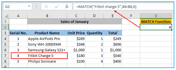
Since “Fitbit Charge 5” is the fourth item, MATCH returns 4. MATCH does not care about case sensitive.
Note: match_type is an important input to the MATCH function. The crucial match_type parameter determines whether matching is precise or approximate. You should frequently use zero (zero) to compel exact match behavior. It’s crucial to supply a value for match_type because the default value of 1, which indicates an approximate match, is used.
2. Using the INDEX Function, lookup and return the cell address
There are a ton of Excel formulas, particularly complex formulas, that use the INDEX function because it is so flexible and powerful. But what does INDEX do in practice? INDEX basically finds the value at a specific position in a range. For illustration, suppose you have a table of the planets in our solar system (see below) and you want to use a method to determine the name of the fourth planet, Jupiter. You can employ INDEX as follows:
=INDEX(A2:A9,4)
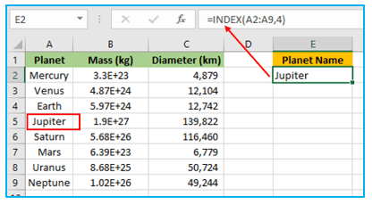
The number from the 4th row of the range is returned by INDEX.
What if you want to use INDEX to calculate Mars’ diameter? In that situation, we can provide a larger range and both a row number and a column number. The INDEX formula below utilizes the entire set of data from A2 to C9 with a row and column number of 4 and 3, respectively:
=INDEX(A2:C9,4,3)
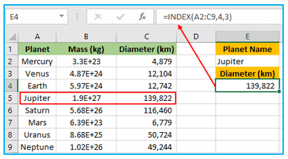
Row 4, column 2, number at INDEX is retrieved.
In summary, INDEX obtains a value based on numeric position at a specific spot in a range of cells. If the range is only one dimension, all you need to provide is a row number. If the range has two dimensions, you must include both the row number and the column number.
You might be contemplating at this moment “Then what? How frequently do you truly know where a cell is located in a spreadsheet?”
True to form. We need a method for determining the location of the items we’re searching for by using the MATCH function, the operation of which is demonstrated above.
3. Using the ADDRESS Function, lookup and return a cell address
This is precisely what Excel ADDRESS formula is designed to do.
It provides you the cell address for that particular cell after taking the row and column numbers.
The syntax of the ADDRESS formula in Excel is as follows:
=ADDRESS(row_num, column_num, [abs_num], [a1], [sheet_text])
where:
row_num: Row number for the cell whose location you’re looking for
column_num: The cell’s column number in which you want the URL is
[abs_num]: You can indicate whether you want the cell reference to be absolute, relative, or mixed using the optional argument.
[a1]: You can indicate in an optional argument whether you want the reference to be in R1C1 style or A1 style.
[sheet_text]: You can indicate in an optional argument whether or not you want to include the sheet name with the cell address.
Let’s use an illustration to demonstrate how this functions now.
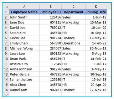
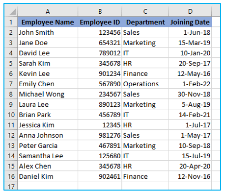
Assume that I have a dataset like the one below, where each employee has a unique employee id, their name, and their department, and I want to quickly find the cell address that includes Emily Chen’s department.
The formula to accomplish this is given below:
=ADDRESS(MATCH(“Emily Chen”,A1:A20,0),3)
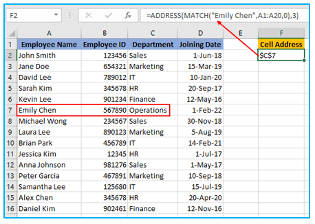
I have used the MATCH function in the formula above to determine the row number that includes the specified employee id.
Additionally, I have used argument number three because the section is listed in column C.
This algorithm has one flaw: it won’t function if you add a row above the dataset or a column to the dataset’s left.
This is so that it won’t alter if I specify the second argument (the column number) as 3, which is a hard-coded value.
The formula would tally 3 columns from the beginning of the worksheet and not from the beginning of the dataset if I added any column to the dataset’s left.
Thus, this will work just fine if you need a straightforward algorithm and a fixed dataset.
However, use the one described in the following part if you require something that is more foolproof.
4. Using the CELL Function, lookup and return the cell address
There is another function that accomplishes the same thing, even though the ADDRESS function was created especially to provide you with the cell reference of the specified row and column number.
Calls itself the CELL function (and it can give you a lot more information about the cell than the ADDRESS function).
The CELL function’s code is listed below:
=CELL(info_type, [reference])
Where:
info_type: The details you require regarding the unit. This could be the file name, location, column number, etc.
[reference]: The cell reference for which you need the cell information is an optional argument that you can give.
How to use CELL formula in Excel to look up and obtain the cell reference is shown below:
Assume you have the dataset depicted below and want to rapidly identify the cell address containing the department for the Emily Chen employee.
The formula to accomplish this is given below:
=CELL(“address”, INDEX($A$1:$D$16,MATCH(“Emily Chen”,$A$1:$A$16,0),3))
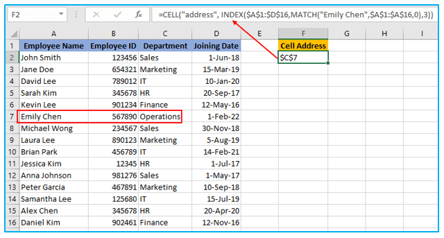
The aforementioned method is very simple.
The second justification I used to determine the department for the employee name Emily Chen was the INDEX algorithm.
I then requested the CELL function to return the cell address for this value, which I had obtained from the INDEX formula, after wrapping it within the CELL function.
The INDEX formula gives the lookup value when you provide it with all the required arguments, and this is the key to understanding how it works. However, it would also return the cell reference for the resulting cell at the same moment.
In our example, the INDEX formula gives the value “Department,” but you can also use it to get the cell reference for that value rather than the actual value.
The INDEX formula typically returns the value when you input it in a cell because that is what is expected of it. However, the INDEX method will provide the cell reference in situations where one is necessary.
That’s precisely what it does in this instance.
The best part of using this formula is that it is not dependent on the worksheet’s first column. This implies that the INDEX formula will still return the right address if you choose any data set (which could be located anywhere in the worksheet).
And the algorithm would change to provide you with the right cell address if you added an extra row or column.
These two straightforward formulas can be used to search up and locate data in Excel and yield the cell address rather than the value.
For ready-to-use Dashboard Templates:
