How to Insert Slicers in Pivot Table?

Insert Slicers in Pivot Table to elevate your data analysis to the next level. By incorporating slicers, you unlock a more dynamic, interactive, and user-friendly approach to data exploration. These tools not only simplify the process of data segmentation and filtering but also enhance the overall clarity and visual appeal of your reports. Embrace the power of slicers to make your pivot tables more accessible and informative, ensuring your data speaks clearly and effectively to all stakeholders. Start leveraging slicers today and transform your data into a compelling narrative that drives informed decisions.

Using Slicers in Pivot Table Excel

When you select one or more options in the Slicer box for a Pivot Table, the data can be filtered. To produce amazing reports, connect several slicers to numerous pivot tables. Slicers offer a more visually appealing method of filtering the Pivot Table data according to the preference.

Inserting slicer in pivot table

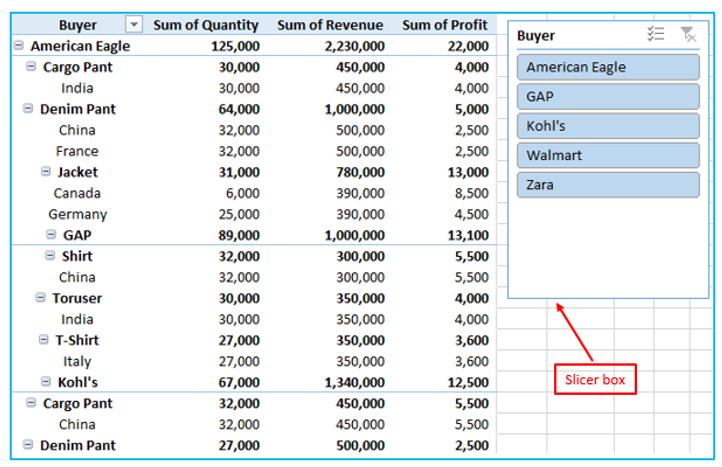
When you only require a portion of the Pivot Table rather than the complete thing, slicers could be needed. You can insert the slicer and rapidly choose the appropriate Buyer Name for which you want to acquire the profit data, for instance, if you just want to see the profits for American Eagle rather than all the buyers.

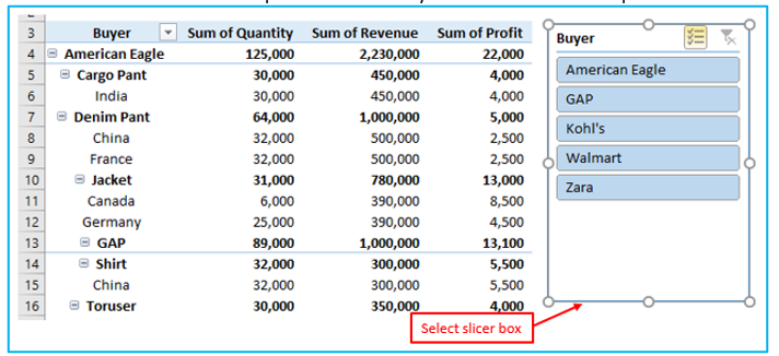
We will use the following sample Pivot Table for demonstration: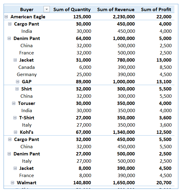

Procedure of inserting slicer in pivot table

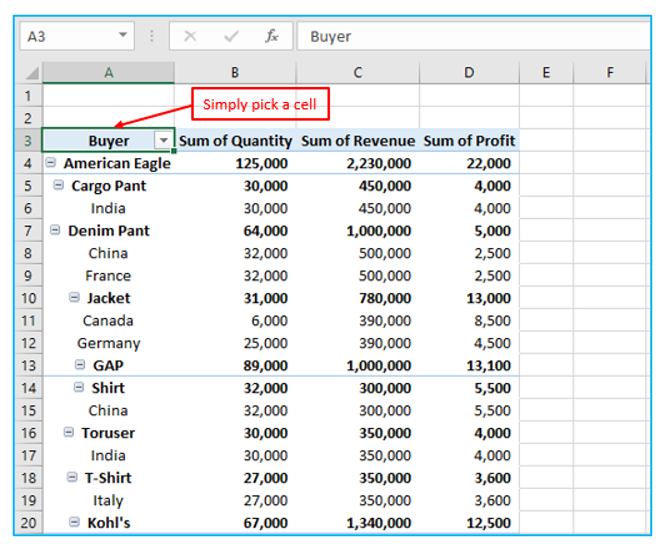
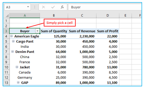
 Step 1: In the Pivot Table, simply pick a cell, outlined in Red below.

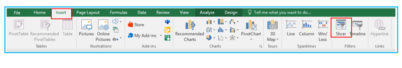
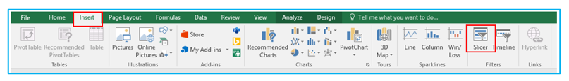
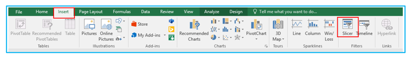
Step 2: Go to “Insert” Tab. Then Select “Slicer”, outlined in Red below.

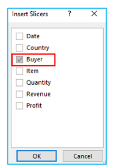
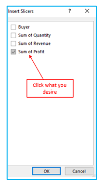
Step 3: Choose the dimension for which you can filter the data in the Insert Slicers dialog box. You can choose one or more dimensions at once from the list of possible dimensions in the Slicer Box. For example, I click only “Buyer”, outlined in Red below.

Step 4: After clicking ok, the result is outlined in Red below.

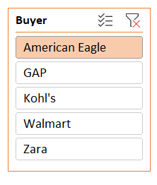
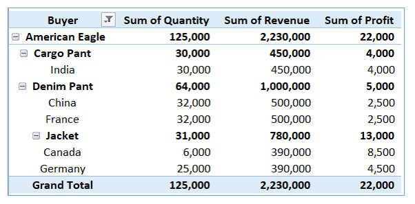
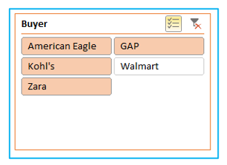
Select ‘American Eagle’ from the Buyer Slicer

In the below table only American Eagle’s data filtered:

Inserting multiple slicers in pivot table:

Additionally, you can enter several slicers by choosing more than one dimension in the Insert Slicers dialog box.

Procedure of inserting multiple slicers in pivot table

Step 1: In the Pivot Table, simply pick a cell, outlined in Red below.

Step 2: Go to “Insert” Tab. Then Select “Slicer”, outlined in Red below

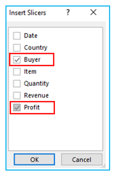
Step 3: Select all the dimensions for which you want the Slicers in the Insert Slicers dialog box. For illustration, I choose “Buyer” and “Profit”, outlined in Red below.

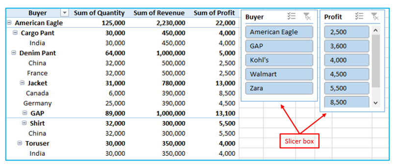
Step 4: After clicking ok, the result is outlined in Red below.

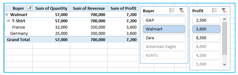
Take note of how these slicers are connected to one another. For instance, if I choose “Walmart” in the Buyer filter and “3,600” in the profit filter, just the profit amount 3,600 information for Walmart customers will be displayed.

Formatting Slice:

When it comes to formatting, a Slicer offers lots of options.

These are the settings that a slicer allows you to change.

Modifying slicer colors:

There are simple ways to change a slicer’s default colors if you don’t like them.

Procedure of modifying slicer color in pivot table:

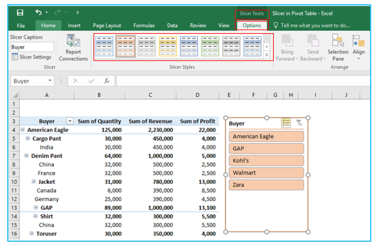
Step 1: Select the slicer, outlined in Red below.

Step 2: Then click Slicer Tools -> Options -> Slicer Styles. There are several possibilities available

Step 2: Then click Slicer Tools -> Options -> Slicer Styles. There are several possibilities available here. Choose the one you want, and your slicer will automatically receive that formatting, outlined in Red below.

Multiple columns in the slicer box:

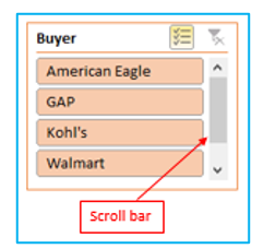
All of the objects from the selected dimension are listed in a Slicer’s default one column, which has one row. Slicer displays a scroll bar if you have a lot of items so you can browse them all, outlined in Red below.

Without the effort of scrolling, you might want to see every item. By developing multiple column Slicer, you may achieve that.

Procedure of creating multiple columns in the slicer box:

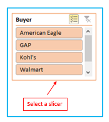
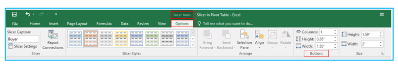
Step 1: Select the slicer, outlined in Red below.

Step 2: Go to “Slicer Tools”, then select “Options” and go to “Buttons”, outlined in Red below.

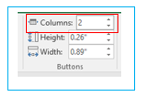
Step 3: Change the Columns value to 2, outlined in Red below.

Step 4: The result looks like below.

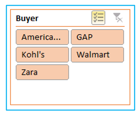
If the names are not presented in their entirety, and it seems cluttered. You can adjust the slicer’s size to improve the appearance. By choosing the slicer and moving the edges with the mouse, you may easily adjust the slicer’s size.

 

Changing/Removing the slicer header:

A Slicer selects the field name from the data by default. For instance, the header would be “Buyer” if I created a slicer for buyer.

You might decide to modify the header or get rid of it entirely.

Procedure of changing/removing the slicer header:

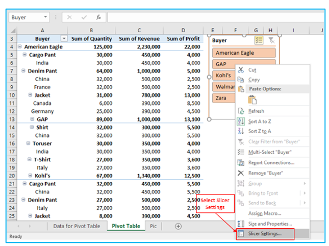
Step 1: Select “Slicer Settings” by performing a right-click on the slicer, outlined in Red below.

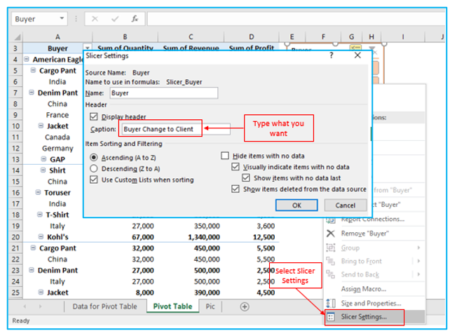
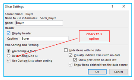
Step 2: Change the header caption to what you want in the Slicer Settings dialog box, then click       ok, outlined in Red below.

 

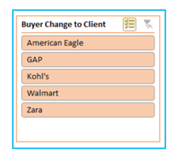
The result looks like below.

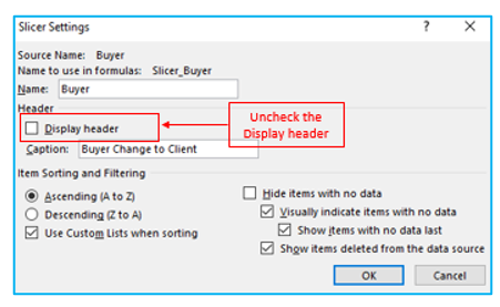
The Display Header option in the dialog box can be unchecked if you don’t want to view the header, outlined in Red below.

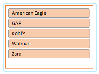
The result looks like below.

 

Sorting Items in the Slicer:

Ascending order for text and Older to Newer for numbers and dates are the default sorting methods for items in Slicers.

The default configuration can be altered, and you can even create your own unique sort criteria.

Procedure of sorting items in the slicer:

Step 1: Select “Slicer Settings” by performing a right-click on the slicer, outlined in Red below.

Step 2: In the Slicer Settings dialog box, you can change the sorting criteria, or use your own unique sorting criteria, outlined in Red below.

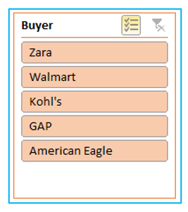
Step 3: After clicking ok, the result looks like below.

Connecting a Slicer to Multiple Pivot Tables:

Multiple Pivot Tables can be attached to a slicer. Once connected, a single Slicer can be used to filter every connected Pivot Table at once.

Remember that the Pivot Tables must share the same Pivot Cache in order to connect them to a Slicer. This indicates that either the same data was used to construct both, or one of the pivot tables was copied and pasted as a different pivot table.

Procedure of connecting a slicer to multiple pivot tables:

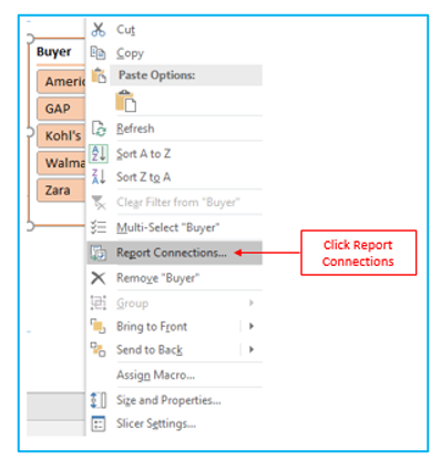
Step 1: Select “Report Connections” by doing a right-click on the Slicer, outlined in Red below

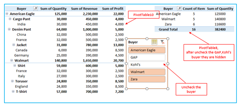
Step 2: You can view the names of all the pivot tables that use the same pivot cache in the Report Connections dialog box. Choose which ones to attach to the Slicer. In this instance, the Slicer is attached to just two Pivot Tables that I have created.

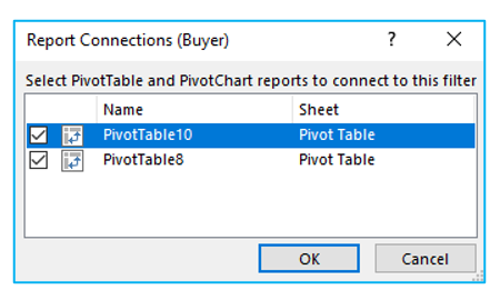
Step 3: After clicking ok, your Slicer is currently linked to both Pivot Tables. Filtering would take place in both Pivot Tables when you made a choice in the Slicer.

Creating Dynamic Pivot Charts using Slicer:

A Slicer can be used with Pivot Charts in the same way that it can be used with Pivot Tables.

Procedure of creating dynamic pivot charts using slicer:

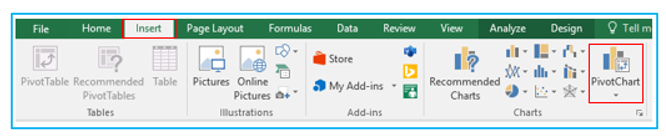
Step 1: Select the data and go to Insert –> Charts –> Pivot Chart, outlined in Red below.

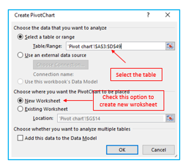
Step 2: Make sure the range is accurate in the Create Pivot Chart dialog box, then click OK. This will create a new sheet with a pivot chart, outlined in Red below.

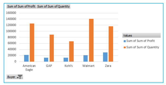
Step 3: To get the Pivot chart you want, choose the fields. I have a chart that displays sum of profit by buyer.

The result looks like below.

Step 4: After getting the Pivot Chart ready, go to Insert –> Slicer.

 

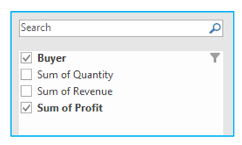
Step 5: With the Chart, choose the Slicer dimension you desire. I check that dimension since I want the profit in this situation, outlined in Red below.

The result looks like below.

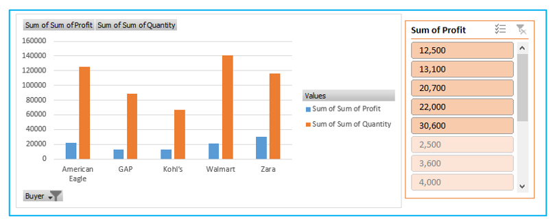
The chart will be changed with your desire filtering in the slicer box.

Keep in mind that you can link many Slicers to a single Pivot Chart and numerous charts to a single Slicer (the same way we connected multiple Pivot Tables to the same Slicer).

Application of Insert Slicers in Pivot Table