Freeze Rows and Columns in Excel to improve your data navigation and enhance productivity. By locking specific rows and columns, you ensure that important headers and labels remain visible as you scroll through your worksheet. Say goodbye to losing track of key information and hello to a more organized and efficient workflow. Whether you’re managing large datasets, creating reports, or analyzing trends, Freeze Rows and Columns in Excel provides a seamless way to keep your critical data in view. Embrace this powerful feature to streamline your tasks, reduce errors, and maintain clarity in your spreadsheets. Elevate your Excel experience by leveraging the convenience and functionality of Freeze Rows and Columns in Excel, ensuring that your data is always accessible and easy to interpret.
This Tutorial Covers:
- How to freeze rows in Excel
- Freeze the top row
- Freeze multiple rows
- How to freeze columns in Excel
- Freeze the first column
- Freeze multiple columns
- Freeze Panes in Excel
- Unfreeze Panes in Excel
- Other view options
- To open a new window for the current workbook
- To split a worksheet
1. How to freeze rows in Excel?
In Excel, freezing rows only requires a few clicks. Depending on how many rows you want to lock, you may simply select one of the following choices by clicking View tab > Freeze Panes:
- Freeze Top Row – to freeze the first row.
- Freeze Panes – to freeze several rows.
The specific instructions are listed below.
-
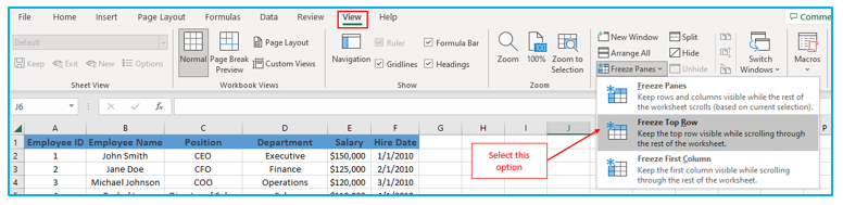
Freeze top row:
By doing this, you may lock the worksheet’s very first row, ensuring that it is always displayed as you move through the other rows.
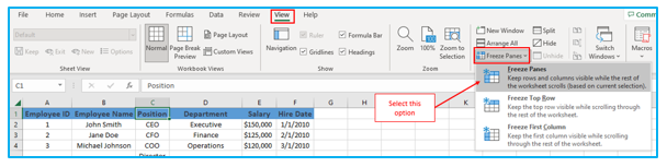
Step 1: Go to the “View” tab, then click “Freeze Panes” under the “Window” group. Then choose “Freeze Top Row”.
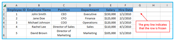
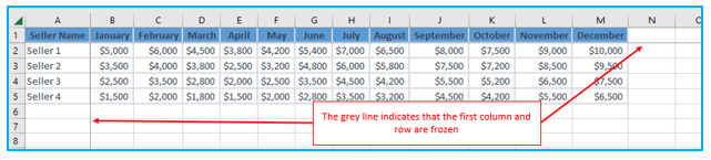
A grey line below the top row indicates that it is frozen:
-
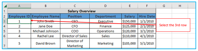
Freeze multiple rows:
If you want to lock multiple rows (beginning with row 1), follow these instructions:
How to freeze rows in excel?
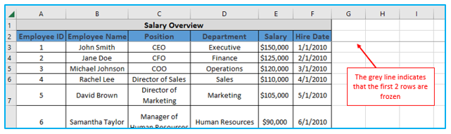
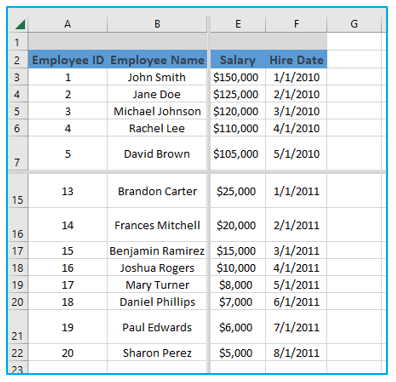
Step 1: In order to freeze a row or rows, select the row beneath it. In this case, we’ll choose row 3 because we wish to freeze rows 1 and 2.
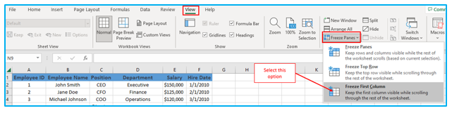
Step 2: Go to the “View” tab, then click “Freeze Panes” under “Window” group. Then choose “Freeze Panes”.
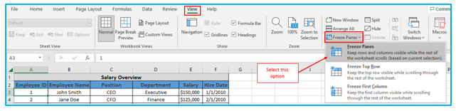
As a result, you can scroll over the sheet’s content while still seeing the first two rows of frozen cells:
Notes:
- In Microsoft Excel, only the rows at the top of the spreadsheet can be frozen. Rows in the center of the sheet cannot be locked.
- Verify that at the time of freezing, all of the rows that need to be locked are visible. If some of the rows are concealed after freezing because they are not visible, they will be. Please refer to How to avoid frozen hidden rows in Excel for more details.
2. How to freeze columns in Excel?
The Freeze Panes instructions in Excel can be used in a similar way to freeze columns.
-
Freeze the first column:
By doing this, the leftmost column will always be visible while you scroll to the right.
How to do freeze excel first column in Excel.
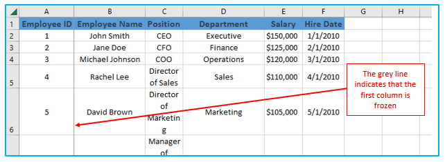
Step 1: Go to the “View” tab, then click “Freeze Panes” under the “Window” group. Then choose “Freeze First Column”.
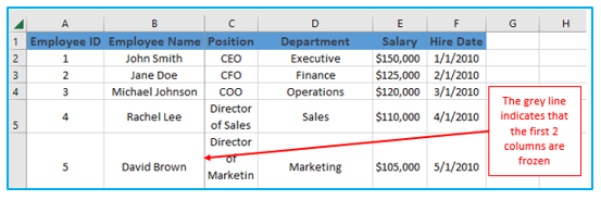
A grey line beside the first column indicates that it is frozen:
-
Freeze multiple columns:
This is what you need to do if you want to freeze more than one column:
Step 1: Choose the column to the right of the last column you want to lock, or the first cell in the column, whichever is appropriate. For instance, choose the entire column C or cell C1 to freeze the first two columns.
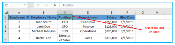
Step 2: Go to the “View” tab, then click “Freeze Panes” under “Window” group. Then choose “Freeze Panes”.
You can examine the cells in the frozen columns as you go across the worksheet since this will lock the first two columns in place, as demonstrated by the thicker and darker border:
Notes:
- Only the left-hand columns of the sheet can be frozen. The worksheet’s center columns cannot be frozen.
- Any columns that are not visible during locking should be visible before locking; any such columns will be hidden after locking.
3. Freeze Panes in Excel:
Microsoft Excel now enables you to freeze both rows and columns simultaneously in addition to locking columns and rows separately. This is how:
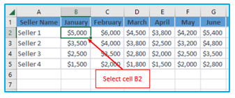
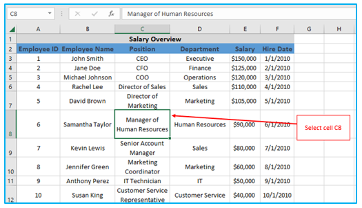
Step 1: Choose a cell that is below the final row and just above the final column that you want to freeze. To freeze the top row and the first column in one action, for instance, choose cell B2.
Step 2: Go to the “View” tab, then click “Freeze Panes” under “Window” group. Then choose “Freeze Panes”.
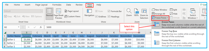
In this manner, as you scroll down and to the right, the header row and leftmost column of your table will always be visible:
In a similar manner, you can freeze any number of rows and columns as long as you begin with the top row and leftmost column. For example, you would choose cell C2 to lock the top row and the first two columns, C3 to lock the first two rows and the first two columns, and so on.
4. Unfreeze Panes in Excel:
You might need to reset the spreadsheet by unfreezing panes in order to choose a different view choice.
The steps to Unfreeze Panes in Excel are described below:
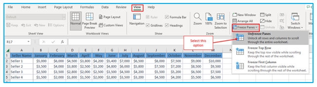
Step 1: Go to the “View” tab, then click “Freeze Panes” under the “Window” group. Then choose ” Unfreeze Panes “.
5. Other view options:
Comparing various portions of a workbook that has a lot of content can occasionally be challenging. Excel has extra features that make it simpler to view and contrast your worksheets. For instance, you can decide to split a worksheet into multiple windows or open your workbook in a new window.
-
To open a new window for the current workbook:
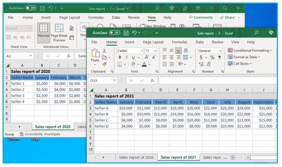
Excel enables you to simultaneously open numerous windows for a single workbook. We’ll compare two separate worksheets from the same workbook using this feature in our example.
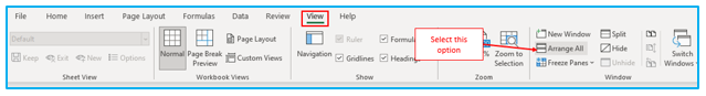
Step 1: Select the New Window option after clicking the Ribbon’s View tab.
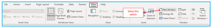
The workbook’s new window will open.
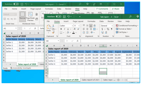
Step 2: Now, worksheets from the same workbook can be compared across windows. To compare sales between 2020 and 2021 in our example, we’ll choose the 2021 Sales Detailed View worksheet.
Use the “Arrange All” command to swiftly reposition any windows that are open at the same moment.
-
To split a worksheet:
Without opening a separate window, you might occasionally want to compare various areas of the same workbook. You can partition the worksheet into numerous panes that scroll independently using the Split command.
Step 1: Choose the cell in which to divide the worksheet. In this instance, we’ll pick cell D5.
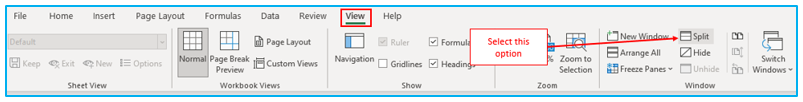
Step 2: Select the Split command by clicking the View tab on the Ribbon.
There will be several panes in the workbook. Using the scroll bars, you can navigate across each pane separately and compare various workbook portions.
You can adjust the size of each segment after making a split by clicking and dragging the vertical and horizontal dividers.
Click the Divide command once more to undo the split.
Application of Freeze Rows and Columns in Excel
- Header Visibility: Keep column headers in view as you scroll down large datasets by freezing the top row, ensuring you always know what each column represents.
- Side Labels: Freeze the first column to maintain visibility of row labels while scrolling horizontally, making it easier to track and reference data.
- Data Comparison: Simplify data comparison by freezing rows and columns that contain key identifiers, allowing you to easily compare data points without losing context.
- Consistent Navigation: Enhance navigation through extensive worksheets by keeping essential information like titles or category names visible at all times, reducing the need for constant scrolling.
- Report Generation: Improve report readability by freezing rows and columns with critical labels and headers, ensuring your reports remain clear and professional.
- Form Templates: Create user-friendly forms and templates by freezing sections that contain instructions or key fields, guiding users through the document without losing important references.
For ready-to-use Dashboard Templates:
