Flip Data in Excel to effortlessly reorganize your datasets and gain new insights. By flipping data, you can reverse the order of rows or columns, making it easier to analyze trends from a different perspective. Say goodbye to manual reorganization and hello to a more efficient way to manage your data. Whether you’re preparing reports, analyzing historical data, or adjusting layouts for better readability, Flip Data in Excel offers a simple yet powerful solution. Embrace the flexibility and convenience of flipping data to enhance your productivity and ensure your data is always presented in the most useful format. Take advantage of this feature to streamline your workflow and make informed decisions with ease.
This Tutorial Covers:
- Flip Data Using SORT and Helper Column
- Vertically flip the data (Reverse Order Upside Down)
- Flip the Data Horizontally
- Flip Data Using Formulas
- Making use of the SORTBY function (available in Microsoft 365)
- Using the INDEX Function
- Flip Data Using VBA
- Flip Data Vertically Using VBA
- Flip Data Horizontally Using VBA
1. Flip Data Using SORT and Helper Column:
Using a helper column and that helper column to sort the data is one of the simplest ways to change the order of the data in Excel.
-
Vertically flip the data (Reverse Order Upside Down):
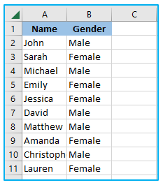
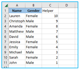
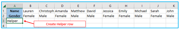
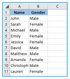
Assume you want to reverse the names in the data set in the A column, as it is displayed below:
The steps to flip the data vertically are as follows:
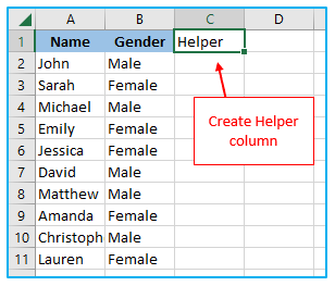
Step 1: Enter “Helper” as the column heading in the adjacent column.
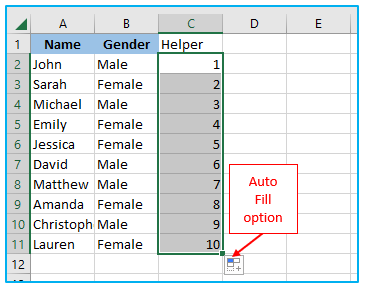
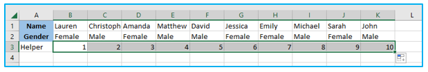
Step 2: Enter several numbers in the helpful column (1, 2, 3, and so on). To accomplish this, use the autofill handle option or fill series option.
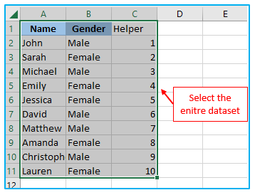
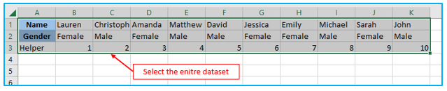
Step 3: Choose the “Helper” column as well as the complete collection of data.
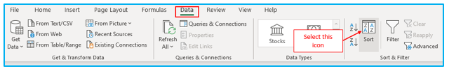
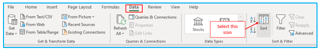
Step 4: Click the “Data” tab. Click on the “Sort” icon under “Sort & Filter” section.
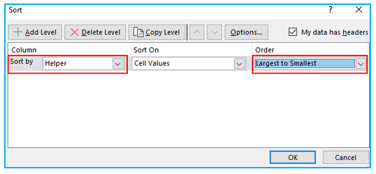
Step 5: Choose ‘Helper’ from the ‘Sort by’ menu in the Sort dialog box. Go to the “Order” drop-down then choose “Largest to Smallest.” After that, click OK.
The aforementioned procedures would reverse the order of the names in the data by sorting the data based on the values of the “Helper” columns.
Feel free to remove the “Helper” column once you’re finished.
In this example, I’ve shown you how to flip the data when there is just one column, but the same method can be applied to a table as a whole. Just be careful to pick the full table before sorting the information in descending order using the helper column.
-
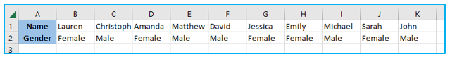
Flip the Data Horizontally:
A similar process may be used in Excel to flip the data horizontally.
Using the Sort dialog box and the “Sort left to right” feature, Excel offers the ability to horizontally sort the data.
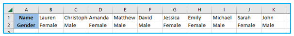
Let’s say you wish to convert the data in the table below from vertical to horizontal.
The procedures are as follows:
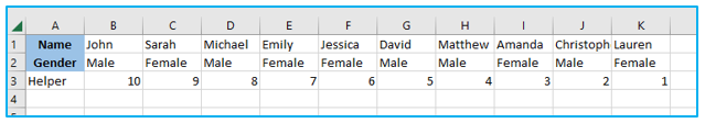
Step 1: Enter “Helper” as the row heading in the row below.
Step 2: Please input a string of numbers in the helper row (1,2,3, and so on).
Step 3: Select the “Helper” row as well as the complete collection of data.
Step 4: Click the “Data” tab. Click on the “Sort” icon under “Sort & Filter” section.
Step 5: Click the “Options…” button in the Sort dialog box.
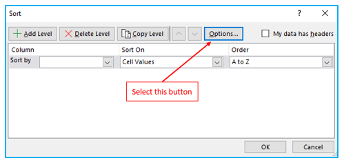
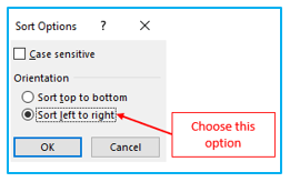
Step 6: Select “Sort left to right” in the dialog box that appears and then press OK.
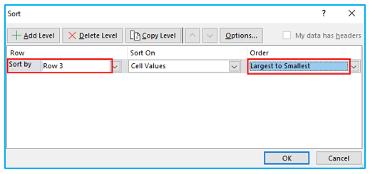
Step 7: Choose Row 3 from the “Sort” by drop-down menu (or whatever row has your helper column). Go to the “Order” drop-down and then choose “Largest to Smallest.” then press OK.
The table would be horizontally flipped if the aforementioned actions were taken.
When finished, you can eliminate the “Helper” row.
2. Flip Data Using Formulas:
The new Excel formulas in Microsoft 365 make it incredibly simple to change the arrangement of a column or table.
In this part, I’ll demonstrate how to accomplish this using either the INDEX formula (if you’re not using Microsoft 365) or the SORTBY formula (if you are).
-
Making use of the SORTBY function (available in Microsoft 365):
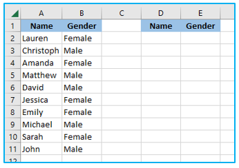
Let’s say you have the table below and wish to flip the information in it:
The steps to flip the data using SORTBY function are as follows:
Step 1: To achieve this, duplicate the headers and set them where the flipped table should be.
Step 2: Apply the formula underneath the cell in the left-most header, which is as follows:
=SORTBY($A$2:$B$11,ROW(A2:A11),-1)
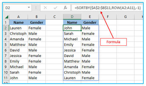
The ROW function result is used as the foundation for sorting the data in the calculation above.
In this scenario, the ROW function would provide an array of numbers that represented the row numbers between the given range (which in this example would be a series of numbers such as 2, 3, 4, and so on).
Additionally, the fact that this formula’s third parameter is a negative number forces the algorithm to sort the data in descending order.
In essence, the order of the data would be reversed, with the record with the highest row number appearing at the top and the record with the lowest rule number appearing at the bottom.
Once finished, you can create a static table by converting the formula to values.
-
Using the INDEX Function:
You can use the incredible INDEX function if you don’t have access to the SORTBY function.
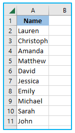
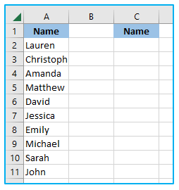
Imagine you wish to flip a dataset of names that looks like the one below.
The steps to flip the data using INDEX function are as follows:
Step 1: To achieve this, duplicate the header and set the header where the flipped table should be.
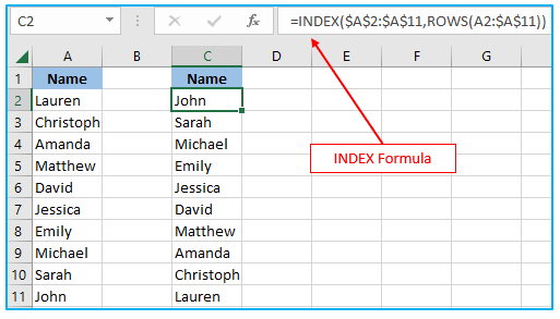
Step 2: Apply the formula underneath the cell in the left-most header, which is as follows:
=INDEX($A$2:$A$11,ROWS(A2:$A$11))
How does this equation function?
The INDEX function is used in the formula above to retrieve the value from the cell based on the second argument’s value.
The second argument, where I utilized the ROWS function, is where the actual magic happens.
The first cell would return the number of rows between A2 and A11, which would be 10, because I had locked the second portion of the reference in the ROWS method.
However, because I have locked it and made it absolute, the initial reference would stay the same as is as it moves along the rows while switching to A3, A4, and so on.
The output of the ROWS function would reduce by 1 as we moved down the rows, from 10 to 9 to 8, and so on.
This would ultimately give us the data in reverse order because the INDEX function returns the result based on the number in the second argument.
Even if the data collection contains numerous columns, you can still use the same formula. However, a second parameter that specifies the column number from which the data must be collected must be provided.
Suppose you wish to flip the order of the complete table and you have the data set as follows:
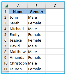
The equation that does that is listed below:
=INDEX($A$2:$B$11,ROWS(A2:$A$11),COLUMNS($A$2:A2))
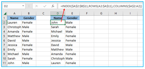
This formula is similar to the previous one, with the addition of a third argument that designates the column number where the value should be fetched.
I’ve used the COLUMNS function to make this formula dynamic, which will continuously change the column value when you copy it to the right from 1 to 2 to 3.
Once finished, you can translate the formulas into values to ensure a static outcome.
Note: Reversing the order of a data set using a formula in Excel will result in the loss of the original formatting. If the sorted data also requires the original formatting, you may either manually apply it or copy and paste the formatting from the original data set.
3. Flip Data Using VBA:
You can also attempt the VBA method if you flip column and row in excel is something you need to do frequently.
A VBA macro code can be copied and pasted once inside the worksheet in the VBA editor before being reused repeatedly inside the same workbook.
To utilize the code in any workbook on your machine, you can alternatively store it as an Excel add-in or in the Personal Macro Workbook.
In the next section, VBA code is provided to flip Excel columns and rows.
-
Flip Data Vertically Using VBA:
The VBA code that would flip the worksheet’s selected data vertically is provided below.
Sub FlipVerically()
Dim Rng As Range
Dim WorkRng As Range
Dim Arr As Variant
Dim i As Integer, j As Integer, k As Integer
On Error Resume Next
xTitleId = “Flip columns vertically”
Set WorkRng = Application.Selection
Set WorkRng = Application.InputBox(“Range”, xTitleId, WorkRng.Address, Type:=8)
Arr = WorkRng.Formula
Application.ScreenUpdating = False
Application.Calculation = xlCalculationManual
For j = 1 To UBound(Arr, 2)
k = UBound(Arr, 1)
For i = 1 To UBound(Arr, 1) / 2
xTemp = Arr(i, j)
Arr(i, j) = Arr(k, j)
Arr(k, j) = xTemp
k = k – 1
Next
Next
WorkRng.Formula = Arr
Application.ScreenUpdating = True
Application.Calculation = xlCalculationAutomatic
End Sub
How to use the Flip Columns macro?
Step 1: Press (Alt + F11) on your keyboard to open the “Microsoft Visual Basic for Applications” window. Paste the aforementioned code into the Code window by selecting Insert > Module.
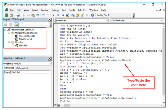
Step 2: Start the macro by pressing F5 on your keyboard. When the Flip Columns dialog appears, choose a range to flip using the prompt. Using the mouse, choose one or more columns (except the column headers), click OK.
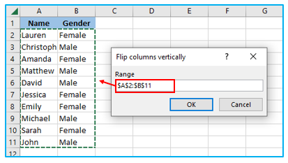
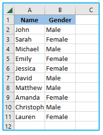
After clicking OK, the outcome will appear shortly.
Make sure to save your file as an Excel worksheet that supports macros in order to save the macro.
-
Flip Data Horizontally Using VBA:
The VBA code that would flip the worksheet’s selected data horizontally is provided below.
Sub FlipDataHorizontally()
Dim Rng As Range
Dim WorkRng As Range
Dim Arr As Variant
Dim i As Integer, j As Integer, k As Integer
On Error Resume Next
xTitleId = “Flip Data Horizontally”
Set WorkRng = Application.Selection
Set WorkRng = Application.InputBox(“Range”, xTitleId, WorkRng.Address, Type:=8)
Arr = WorkRng.Formula
Application.ScreenUpdating = False
Application.Calculation = xlCalculationManual
For i = 1 To UBound(Arr, 1)
k = UBound(Arr, 2)
For j = 1 To UBound(Arr, 2) / 2
xTemp = Arr(i, j)
Arr(i, j) = Arr(i, k)
Arr(i, k) = xTemp
k = k – 1
Next
Next
WorkRng.Formula = Arr
Application.ScreenUpdating = True
Application.Calculation = xlCalculationAutomatic
End Sub
Follow the instructions above to use the macro to your Excel workbook. The next dialog window will appear when you execute the macro and ask you to choose a range. Click OK after selecting the full table, excluding the header row.
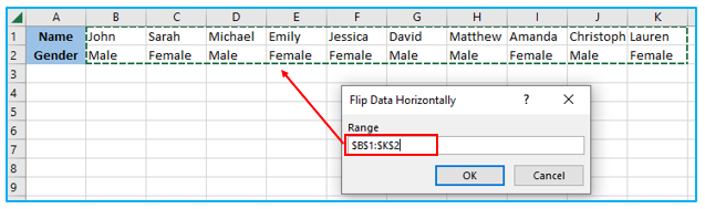
In a split second, the rows’ data order was reversed:
These are some techniques you can employ in Excel to flip the data (i.e., reverse the order of the data set).
Both column row excel data flipping may be accomplished using the techniques I’ve discussed in this lesson (formulas, the SORT feature, and VBA).
I sincerely hope this tutorial was helpful.
Application of Flip Data in Excel
- Transpose Tables: Flip Data in Excel to transpose tables, converting rows into columns and vice versa, facilitating data analysis and presentation.
- Change Data Orientation: Reverse the order of rows or columns to change the orientation of data, providing a different perspective for analysis or visualization.
- Adjust Layouts: Rearrange data layouts by flipping rows or columns to reorganize information and improve the clarity and readability of spreadsheets.
- Pivot Data: Pivot data by flipping rows and columns to transform datasets into pivot tables, allowing for dynamic analysis and exploration of data relationships.
- Combine Data: Merge multiple datasets by flipping and aligning rows or columns, enabling comprehensive analysis and comparison of related information.
- Data Cleaning: Use Flip Data in Excel to clean and standardize datasets by rearranging information into a consistent format, enhancing data quality and usability.
For ready-to-use Dashboard Templates:
