Finding the top 10 values in Excel is a popular way to present data, particularly on dashboards and compiled reports. A top list is used to rate businesses or people according to their values. In this tutorial, we will learn about some formulas for finding the top 10 values in an Excel worksheet.
This Content Covers:
- How to Find Top 10 Values in Excel using Dynamic array Formulas?
- By combining the INDEX, SORT, and SEQUENCE functions (Excel 2021 & Excel 365)
- By Combining the CHOOSECOLS, CHOOSEROWS, SORT, and SEQUENCE functions (Excel 365 only)
- How to Find Top 10 Values in Excel using Dynamic Arrays with Criteria?
- Using FILTER Function with INDEX, SORT and SEQUENCE Function
- Using FILTER Function with CHOOSEROWS, CHOOSECOLS
- Calculating Top Values Based on Multiple Criteria
- How to Find the Top 10 Values in Excel using Traditional Functions?
- Using the LARGE Function
- Identify the Labels When the Top 10 Values are Not Unique
- Top 10 Values using Single Criteria
- Top 10 Values using Multiple Criteria
- How to Find the Bottom 10 Values in Excel using Formulas?
- Bottom 10 Values using Dynamic Array Formulas
- Bottom 10 Values using Traditional Formulas
1. How to Find Top 10 Values in Excel using Dynamic array Formulas?
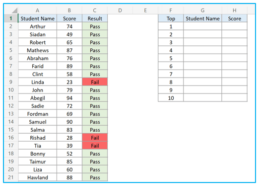
Suppose we have a table like this which contain the data of students, their scores, and result. But the data here are not sorted and we want to find the top 10 scores and their scorer among these students.
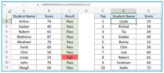
1.1 By combining the INDEX, SORT, and SEQUENCE functions (Excel 2021 & Excel 365)
Step 1: Select cell G2 and insert the following formula in this cell.
=INDEX(SORT(A2:C21,2,-1),SEQUENCE(10),{1,2})
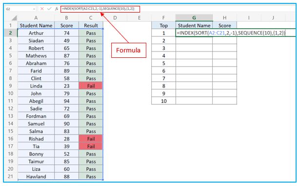
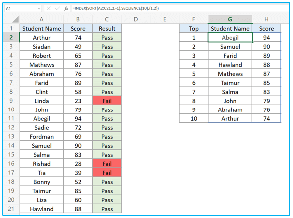
Step 2: Press ENTER key. When you press the ENTER key the formula will return you the top 10 scores and their scorer data. There is no need to auto-fill or insert the formula in multiple cells, you just have to insert it in one cell, and done, you got your result.
Formula Breakdown:
SEQUENCE(10)- The number of rows, columns or data to return. The SEQUENCE function in our example generates a list of numbers from 1 to 10.
SORT(A2:C21,2,-1)- The SORT function in our example looks through the range or criteria A2:C21 to sort. 2 is the sort index here which means the function will sort the data based on column B/column 2. Use 1 to sort in ascending order and -1 for descending order.
INDEX(SORT(A2:C21,2,-1),SEQUENCE(10),{1,2})- Uses SORT and SEQUENCE functions and (1,2) returns the data of column 1 and 2.
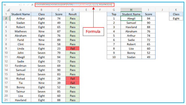
1.2 By Combining the CHOOSECOLS, CHOOSEROWS, SORT, and SEQUENCE functions (Excel 365 only)
Step 1: Insert the following formula into cell G2 after choosing this cell.
=CHOOSEROWS(CHOOSECOLS(SORT(A2:C21,2,-1),1,2),SEQUENCE(10))
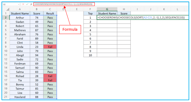
Step 2: Press ENTER key.
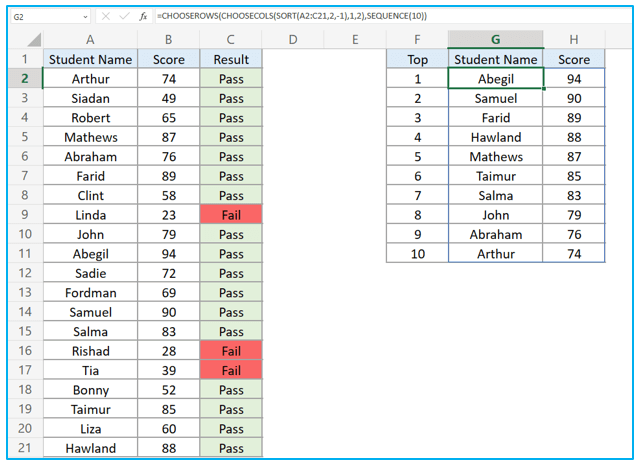
Formula Breakdown:
CHOOSECOLS(SORT(A2:C21,2,-1),1,2)- Column 1 and 2 are returned after the values from cells A2:C21 are sorted by column 2 in decreasing order.
CHOOSEROWS(CHOOSECOLS(SORT(A2:C21,2,-1),1,2),SEQUENCE(10))- This only returns the top 10 rows of the previous CHOOSECOLS result.
2. How to Find Top 10 Values in Excel using Dynamic Arrays with Criteria?
2.1 Using FILTER Function with INDEX, SORT, and SEQUENCE Function
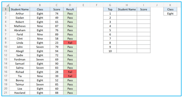
Now we have a situation where the students are from different classes and we want to get the top 10 values only for class eight students.
Step 1: Insert the below given formula inside H2.
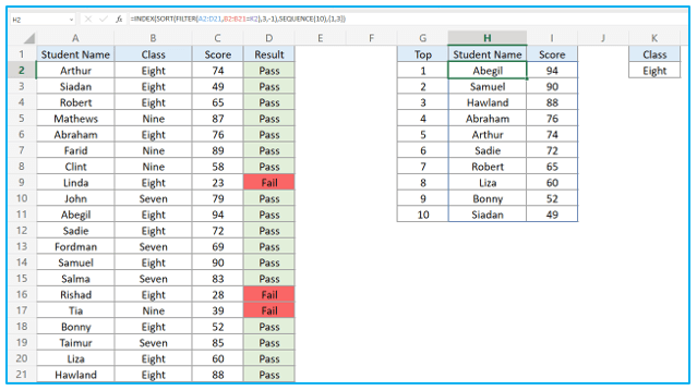
=INDEX(SORT(FILTER(A2:D21,B2:B21=K2),3,-1),SEQUENCE(10),{1,3})
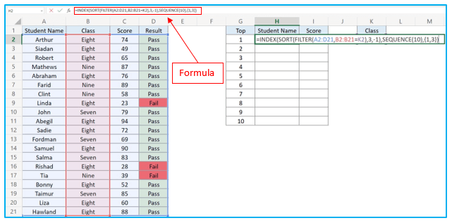
Step 2: Hit the ENTER key and this formula will return you the top 10 values based on a criteria. you choose. The FILTER function here returns cells A2 to D21, but only where the corresponding values from B2 to B21 equal the selected class in cell K2.
2.2 Using FILTER Function with CHOOSEROWS, CHOOSECOLS
Step 1: Place the following formula into H2 and hit ENTER key. This works in Excel 365 only.
=CHOOSEROWS(CHOOSECOLS(SORT(FILTER(A2:D21,B2:B21=K2),3,-1),1,3), SEQUENCE(10))
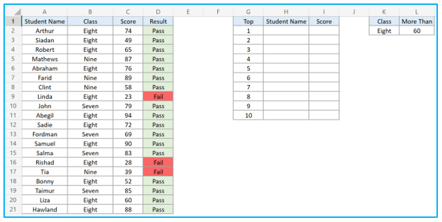
2.3 Calculating Top Values Based on Multiple Criteria
Here we have two conditions, the students have to be from class eight and their score must be more than 60. Now we will see how we can look for the top 5 scorers from this list of students who scored more than 60 and are in class eight.
Step 1: Input the given formula in H1 and press ENTER.
=INDEX(SORT(FILTER(A2:D21,(B2:B21=K2)*(C2:C21>L2)),3,-1), SEQUENCE(5),{1,3})
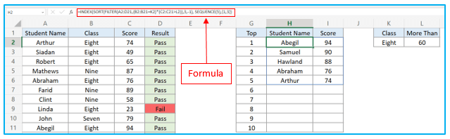
The FILTER function is essential when working with multiple criteria. While using FILTER function on multiple criteria, the plus sign (+) generates OR logic, whereas the asterisk (*) creates AND logic.
3.How to Find Top 10 Values in Excel using Traditional Functions?
3.1 Using the LARGE Function
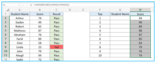
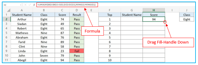
Step 1: Select cell H2 and insert the below given formula in this cell. Press ENTER.
=LARGE($B$2:$B$21,ROW(G2)-ROW(G$1))
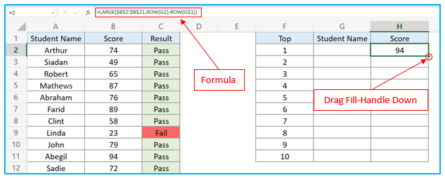
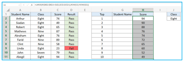
Step 2: Drag the fill handle downwards to apply the formula in the other cells of this column. This will return the top 10 values/scores from this data table.
The LARGE function [=LARGE(range,k)] has two arguments, range and k. When we used the LARGE function in cell H2, it looked through the range $B$2:$B$21 to sort the values. ROW($G$2)-ROW($G$1) here is the “k”( the Nth item to be found ). So, the first row of data calculates as 1, the second row calculates as 2, and so on.
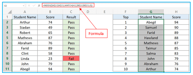
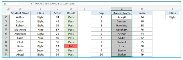
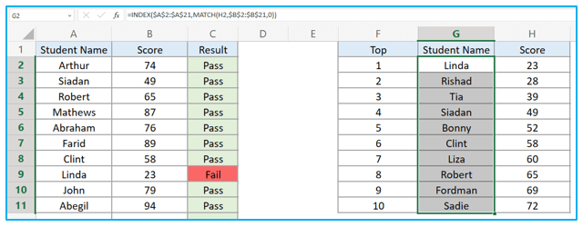
Step 3: Now we will use the INDEX and MATCH functions to find the labels or the scorers for the top 10. Insert this formula in G2 and drag it downwards.
=INDEX($A$2:$A$21,MATCH(H2,$B$2:$B$21,0))
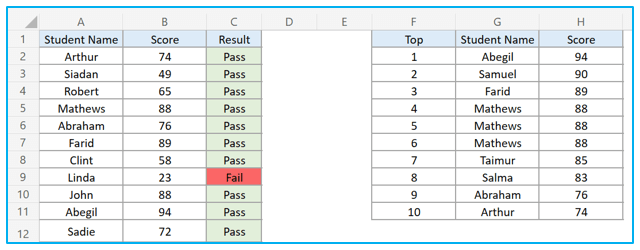
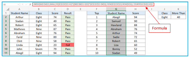
3.2 Identify the Labels When the Top 10 Values are Not Unique
Suppose we got a situation where the top 10 values/scores are not unique and three of the students scored the same score 88. In this sort of situation, finding the labels is tough because a basic INDEX/MATCH function only returns the first value so it finds the name Mathews thrice. Though John and Hawland also scored 88 but their names aren’t in the list. We will have to use an advanced array formula to solve this issue.
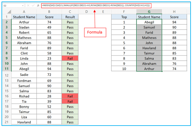
Step 1: Insert the formula in G2 after selecting it and hit ENTER key. Drag the cell down from G2 to G11.
=INDEX($A$2:$A$21,SMALL(IF($B$2:$B$21=H2,ROW($B$2:$B$21)-ROW($B$1)), COUNTIF($H$2:H2,H2)))
Formula Breakdown:
SMALL- The SMALL function looks for the Nth smallest value inside the criteria. It works quite similar to LARGE function, the only difference being it looks for the smallest values.
IF- IF($B$2:$B$21=H2,ROW($B$2:$B$21)-ROW($B$1))
If B2 = H2 then return the count of rows between B2 and B1.
This formula is an array; therefore, it automatically moves on to the next row and does another calculation.
If B3 = H2 then return the count of rows between B3 and B1.
This process goes on.
The IF function’s calculation for the formula in G2 matches the 10th item/student name from the list. So, the only value that is True is 10th item.
COUNTIF– COUNTIF identifies the number of times the value has already occurred in the top 10. Only 1 item in the top 10 for the first row has a score of 94, thus COUNTIF will calculate as 1.
Since all other results are FALSE, the SMALL function will only discover the first smallest number which is 10.
The INDEX function is then used to find the 10th value in the source table. Finally, the result for this calculation is found in cell A11, which is Abegil in this instance. The we just drag G2 downwards to apply the formula in the other cells to get the labels for you top 10 values.
3.3 Top 10 Values Based on Single Criteria
Step 1: Now we will find the top 10 values/scores for class eight only using the traditional function. Insert the formula in H2 and hit Enter key.
=LARGE(IF($B$2:$B$21=$J$2,$C$2:$C$21),ROW(G2)-ROW(G$1))
Step 2: Drag the fill handle downwards and the formula will return the top 10 scores by class eight students.
Step 3: Use any of the methods shown before to find the labels for these top 10 values.
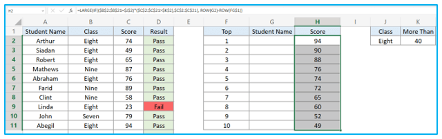
3.4 Top 10 Values Based on Multiple Criteria
Step 1: Select cell H2 and insert the following formula inside the cell and hit Enter key.
=LARGE(IF(($B$2:$B$21=$J$2)*($C$2:$C$21>$K$2),$C$2:$C$21), ROW(G2)-ROW(FG$1))
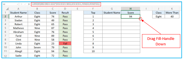
Step 2: Drag the fill handle how to input the formula in the other cells also. This formula will return the top 10 scores that are more than 40 and scored by the students of class eight.
Step 3: Now select cell G2 and incorporate the following formula in it. Drag the cells downwards and you will get the labels for these 10 values.
=INDEX($A$2:$A$21,SMALL( IF(($C$2:$C$21=H2)*(($B$2:$B$21=$J$2)*($C$2:$C$21>$K$2)), ROW($C$2:$C$21)-ROW($C$1)), COUNTIF(H2:$H$2,H2)))
4.How to Find Bottom 10 Values in Excel using Formulas?
4.1 Bottom 10 Values using Dynamic Array Formulas
Step 1: In this tutorial, we saw some dynamic array formulas and used them to get the top 10 values from a data table. Now to find the bottom 10 values, all we will have to do is make a small change inside the SORT function and use “1” instead of “-1”. This will sort the list in ascending order and return us the bottom 10 values as you can see in the picture below.
4.2 Bottom 10 Values using Traditional Formulas
Step 1: To find the bottom 10 values using a traditional formula, simply use SMALL function in place of or LARGE function.
=SMALL($B$2:$B$21,ROW(G2)-ROW(G$1))
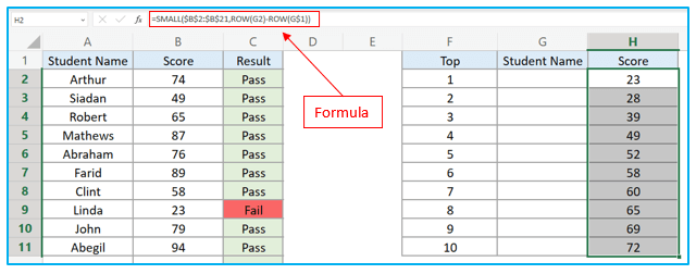
Step 2: Then find labels for you bottom 10 values using any of the methods shown before.
For ready-to-use Dashboard Templates:
