Extract numbers from strings in Excel to streamline data processing and ensure accurate numerical analysis, a task crucial for data analysts, accountants, and anyone dealing with mixed-format data. Whether you’re parsing product codes, extracting quantities from inventory lists, or analyzing data with embedded numbers, mastering this skill is essential. This guide will provide you with a step-by-step approach to efficiently extract numbers from strings in Excel, utilizing formulas and functions to separate numerical data from text. By honing this technique, you’ll enhance the precision of your data manipulation, ensuring that your analysis is based on accurate, number-specific insights.
How to extract numbers from the beginning of a text?
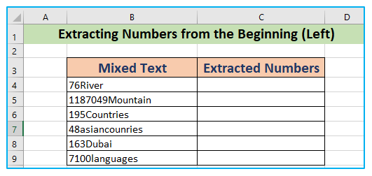
In below table, each cell contains a combination of text and numbers, with the number always appearing at the start of the content. To get the number, use the following formula:
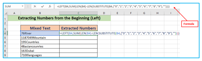
=LEFT(B4,SUM(LEN(B4)-LEN(SUBSTITUTE(B4,{“0″,”1″,”2″,”3″,”4″,”5″,”6″,”7″,”8″,”9″},””))))
Step 1: Prepare a data table with information:
Step 2: Set the formula in cell C-4:
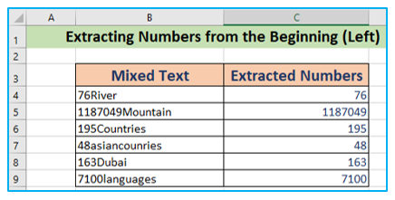
Step 3: Press ENTER and drag Fill Handle to use it to the other cell. Result outlined below:
How this formula works:
- SUBSTITUTE(B4,{“0″,”1″,”2″,”3″,”4″,”5″,”6″,”7″,”8″,”9″},””)
The SUBSTITUTE function will look for successive digits (0-9) and, if found, will replace that digit in cell B4 with an empty character every time. As a result, the function will return- {“76River”,” 76River”,” 76River”,” 76River”,” 76River”,” 76River”,” 7River”,” 6River”,” 76River”,” 76River”}.
- LEN(SUBSTITUTE(B4,{“0″,”1″,”2″,”3″,”4″,”5″,”6″,”7″,”8″,”9″},””))
The LEN function returns the number of characters in a string. As a result, the LEN function will count all the characters discovered separately in the texts via the SUBSTITUTE function. In our example, the resulting values will be – {7,7,7,7,7,7,6,6,7,7}.
- LEN(B4)-LEN(SUBSTITUTE(B4,{“0″,”1″,”2″,”3″,”4″,”5″,”6″,”7″,”8″,”9″},””))
This phase of the calculation involves subtracting the number of characters in cell B4 from all other numbers of characters found individually in the preceding section of the formula. As a result, the resulting values will be – {0,0,0,0,0,0,1,1,0,0}.
- SUM(LEN(B4)-LEN(SUBSTITUTE(B4,{“0″,”1″,”2″,”3″,”4″,”5″,”6″,”7″,”8″,”9″},””)))
The SUM function will then simply add all of the subtracted values found, yielding the following result 2.
- =LEFT(B4,SUM(LEN(B4)-LEN(SUBSTITUTE(B4,{“0″,”1″,”2″,”3″,”4″,”5″,”6″,”7″,”8″,”9″},””))))
Now comes the final component of the formula, where the LEFT function will return values with an exact number of characters from the left found in the previous section. Because the sum value is 2, the LEFT function will only return 76 from the string 76River.
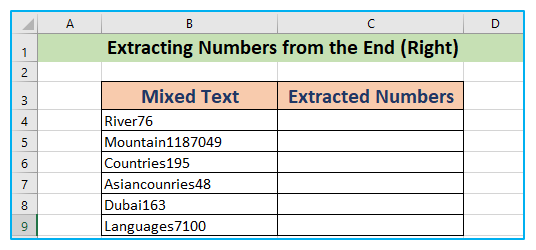
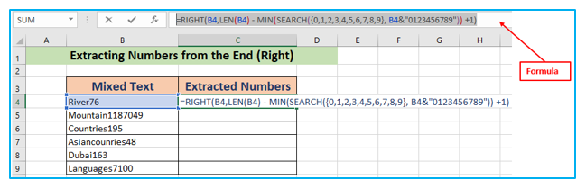
How to extract numbers from the right side of a text? How to extract numbers from string in excel – end of the text?
If you have a column of alphanumeric strings where the number comes after the text, you can use the formula below to get it.
To get the number, use the following formula:
=RIGHT(B4,LEN(B4) – MIN(SEARCH({0,1,2,3,4,5,6,7,8,9}, B4&”0123456789″)) +1)
Step 1: Prepare a data table with information:
Step 2: Set the formula in cell C-4:
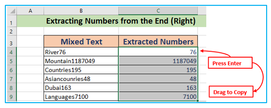
Step 3: Press ENTER and drag Fill Handle to use the formula to the other cell. Result outlined below:
How this formula works:
- B4&”0123456789″
We’re concatenating numbers in the B4 cell with 0123456789 by putting an ampersand (&) between them, and the result is-River760123456789.
- SEARCH({0,1,2,3,4,5,6,7,8,9}, B4&”0123456789″)
The SEARCH function will now search for all digits (0-9) one by one in the resultant value acquired in the previous section and provide the places of those ten digits in the characters of River760123456789. As a result, our final values will be- {8,9,10,11,12,13,7,6,16,17}.
- MIN(SEARCH({0,1,2,3,4,5,6,7,8,9}, B4&”0123456789″))
The MIN function returns the array’s lowest digit or number. So, the least or lowest number will be 6 from the array 8,9,10,11,12,13,7,6,16,17 given in the preceding section of the formula.
- LEN(B4)-MIN(SEARCH({0,1,2,3,4,5,6,7,8,9},B4&”0123456789″))+1
The LEN function will now determine the number of characters in B4. Then it will deduct the value 6 (found in the previous step) and then add 1 to the result. In this situation, the resultant value is 2.
- RIGHT(B4,LEN(B4) – MIN(SEARCH({0,1,2,3,4,5,6,7,8,9}, B4&”0123456789″)) +1)
The RIGHT function returns the number of characters supplied from the string’s final or right side. Following the outcome of the subtraction operation in the preceding section, the RIGHT function will display the last two characters from column B4, which is 76.
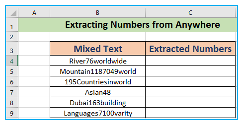
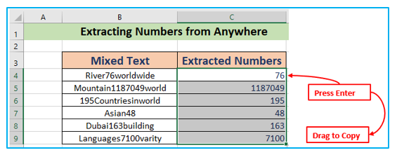
How to extract numbers from mixed text when number can be anywhere in the text?
Finally, consider the case when the numbers can appear anywhere in the text, whether at the beginning, end, or center.
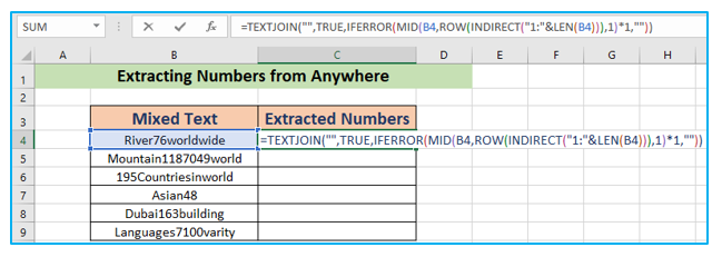
To get the number, use the following formula:
=TEXTJOIN(“”,TRUE,IFERROR(MID(B4,ROW(INDIRECT(“1:”&LEN(B4))),1)*1,””))
TEXTJOIN Function available in Office 2019 and Microsoft 365.
Step 1: Prepare a data table with information:
Step 2: Set the formula in cell C-4:
Step 3: Press ENTER and drag Fill Handle to use the formula to the other cell. Result outlined below:
How this formula works:
Let us break this formula to better understand it. We will proceed from the inner to the exterior functions:
- LEN(B4)
This function returns the length of the string in cell B4. In our case, it yields 16
- INDIRECT(“1:”&LEN(B4))
This function just returns a reference to all rows from 1 to 12.
- ROW(INDIRECT(“1:”&LEN(B4)))
This function just provides a list of numbers ranging from 1 to 12. As a result, the following array is returned by this function:
{1;2;3;4;5;6;7;8;9;10;11;12;13;14;15;16}
Note: We want to be able to customize this formula based on the length of the string being worked on. This ensures that the function is adjusted when copied to another cell.
- MID(B4,ROW(INDIRECT(“1:”&LEN(B4))),1)
Following that, the MID function pulls the character from B4 that corresponds to each position in the array. In other words, it returns an array in which each character of the text in B4 is represented as a single element, as shown below:
{“r”;”i”;”v”;”e”;”r”;”7”;”6″;”w″;”o″;”r”;”l”;”d”;”w”;”i”;”d”;”e”}
- IFERROR(MID(B4,ROW(INDIRECT(“1:”&LEN(B4))),1)*1,””)
The IFERROR function removes all #VALUE! errors, leaving only the digits. This part’s output might look like this –
{“”;””;””;””;””;”7”;”6″;”″;”″;””;””;””;””;””;””;””}
- TEXTJOIN(“”,TRUE,IFERROR(MID(B4,ROW(INDIRECT(“1:”&LEN(B4))),1)*1,””))
The TEXTJOIN function here combines the remaining string characters (which are merely numbers) and ignores the empty string characters. Finally, we receive the number characters in the combined text, “76.”
For ready-to-use Dashboard Templates:
