Display Text in Pivot Table Values Area to elevate the clarity and effectiveness of your data analysis. By incorporating textual data alongside numerical insights, you create a more comprehensive and accessible report that speaks to a wider audience. Whether it’s summarizing data categories, highlighting key findings, or indicating data quality, using text transforms your pivot tables into more informative, actionable tools. Master the skill of displaying text in the pivot table values area to unlock new dimensions in your Excel reports and dashboards.
This Content Covers:
- How to Display Text in Pivot Table Values Area using Data Model?
- How to Display Text in Pivot Table Values Area using Conditional Formatting?
1. How to Display Text in Pivot Table Values Area using Data Model?
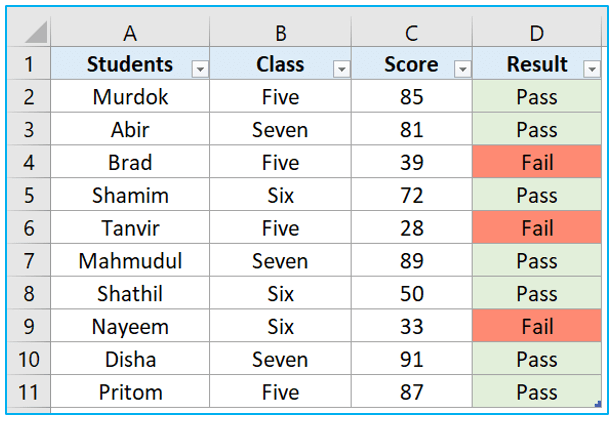
Suppose we have this data table and we want to show the students’ names in the values area. Normally if we put the students category in the values area, it will give us the count of students. Now we will see how we can display the students’ names as text, instead of count inside Pivot table values area using the data model.
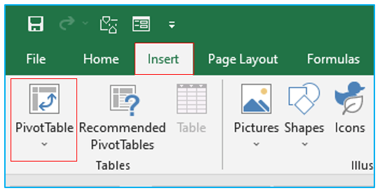
Step 1: Select the data-table and go to Insert>>Pivot Table.
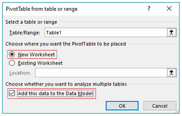
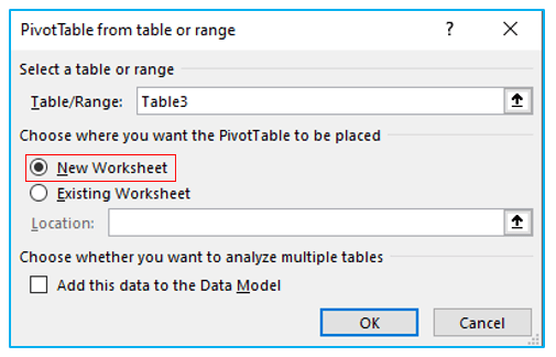
Step 2: This Pivot Table dialogue box will appear in your screen. Choose New Worksheet and check the box (Add this data to the Data Model). Click Ok.
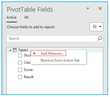
Step 3: A new worksheet will open in your workbook. From PivotTable Fields, right on the table name and choose Add Measure.
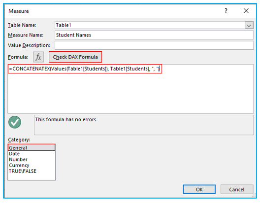
Step 4: The Measure dialogue box will pop up. Type a name inside Measure Name box and insert the following formula inside Formula box. From the Category list, keep it to General. Click on Check Dax Formula to see if there are any errors in the formula or not. If the formula is fine then press OK.
=CONCATENATEX(Values(Table1[Students]), Table1[Students], “, “)
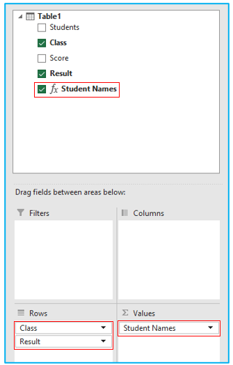
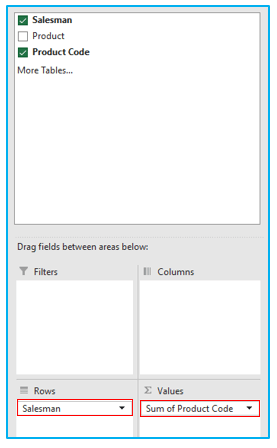
Step 5: Inside the PivotTable Fields there is now a new option added (Student Names) that we just created from Measure box. Drag Student Names inside Values field and drag Class and Result inside Rows field.
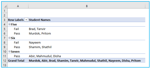
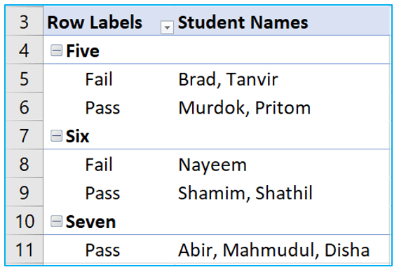
Step 6: The pivot table is created and it looks like this, where the texts are inside Values area. To give it a better look we will remove the grand total from this table.
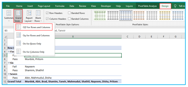
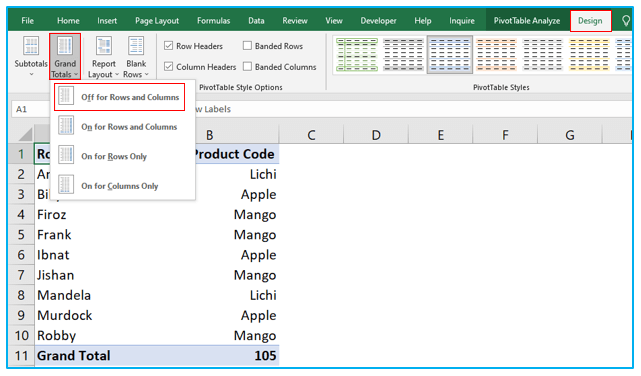
Step 7: Click on the table and go to Design>>Grand Totals and select Off for Rows and Columns from the drop-down list.
Step 8: The table will look like this after removing the grand total.
2. How to Display Text in Pivot Table Values Area using Conditional Formatting?
Now we will see how we can display text in pivot table values area by using conditional formatting.
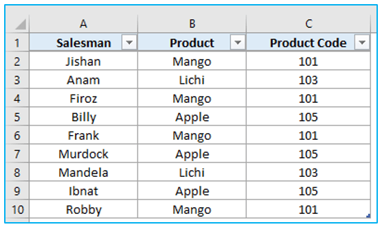
Step 1: First we have to create a pivot table by using the data above. Select the table and go to Insert>>Pivot Table. From the Pivot Table dialogue box, choose New Worksheet and keep the Add this data to the Data Model box unchecked. Click OK.
Step 2: Drag Salesman inside Rows field and Product Code inside Values field.
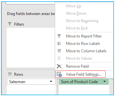
Step 3: Click on Sum of Product Code and go to Value Field Settings.
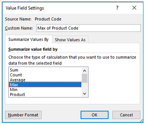
Step 4: Select Max from Summarize values field by category and click OK.
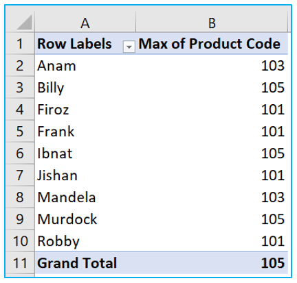
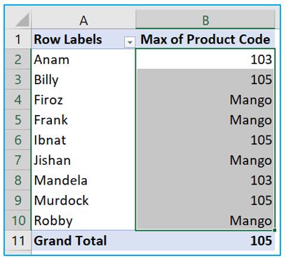
Step 5: This is our pivot table now where the product code has three values (101,103,105).
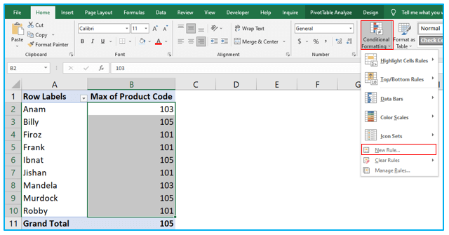
Step 6: Now we will change these values into text. For that select the range (B2:B10) and go to Home>>Conditional Formatting>>New Rules.
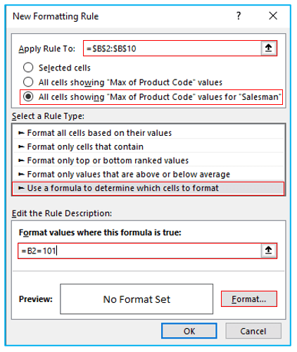
Step 7: The New Formatting Rule dialogue box will appear on your screen. Select the third option from the first box (All cells showing “Max of Product Code” values for “Salesman”) and input the range inside Apply Rule To box. Then select Use a formula to determine which cells to format from the Select a Rule Type box. Inside the formula box, type this formula, =B2=101. After all these are done, click on Format option which is at the bottom right of this dialogue box.
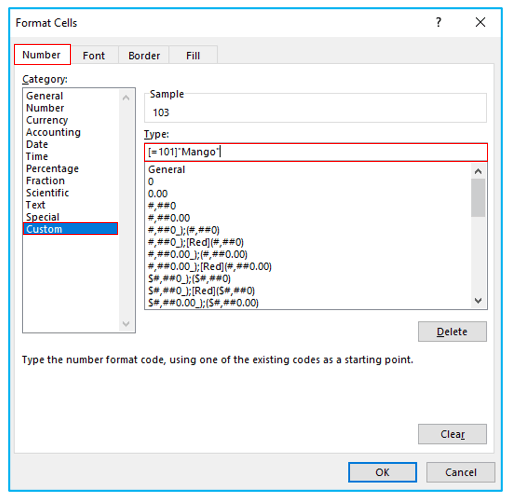
Step 8: From the Format Cells dialogue box, go to Number tab>>Custom. Now type this, [=101]”Mango” inside Type box.
Step 9: Click OK>>OK. All the Product codes 101 which was for the product Mango are now changed into text.
Step 10: To change the other two product codes into product names, simply follow Step 6-9 again.
To change product 103 into Lichi, use =B2=103 inside New Formatting Rule dialogue box and type [=103]”Lichi” inside the Type box in Format Cells prompt.
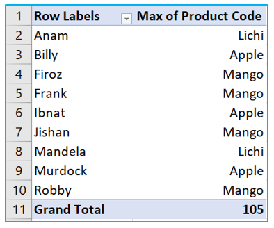
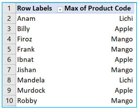
To change product 105 into Apple, use =B2=105 inside New Formatting Rule dialogue box and type [=105]” Apple” inside the Type box in Format Cells prompt. When you are done, the pivot table will look like this.
Step 11: To remove the Grand Total, select the table and go to Design>>Grand Totals>>Off for Rows and Columns.
Step 12: Final result.
Application of Display Text in Pivot Table Values Area
For ready-to-use Dashboard Templates:
