Dynamic Named Range in Excel revolutionizes your approach to data management, offering a fluid, adaptable method to reference data ranges that evolve as your data grows or changes. This advanced feature not only simplifies your formulas but also ensures that your analyses, charts, and dashboards automatically reflect the most current data. Embrace the flexibility and precision of Dynamic Named Range in Excel to elevate your spreadsheets, making them more intuitive, responsive, and powerful tools in your data analysis toolkit.
In this tutorial, we will show you how to create and use a Dynamic Named Range in Excel. Whether you’re a beginner or an experienced Excel user, this tutorial will guide you through the process step-by-step, so you can start using this feature to manage your data more effectively.
This Tutorial Covers:
- What Does Excel Dynamic Named Range Mean
- Why should we use a dynamic named range in Excel
- How to Create Excel Dynamic Named Range (Step by Step)
- Rules for Creating Dynamic Named Range in Excel
1. What Does Excel Dynamic Named Range Mean?
Dynamic Named Range in Excel is a range of cells that adjusts automatically as the data within the range changes, making it a dynamic range. These ranges can be associated with dashboards, charts, or reports. We can create a dynamic named range by naming the range from the name box. For instance, to create a table as a dynamic named range, we need to select the “Data,” insert a table and then give it a name. This tutorial will guide you through the process of creating and using dynamic named ranges in Excel.
2. Why should we use a dynamic named range in Excel?
Naming ranges in Excel can be incredibly useful for a variety of reasons. Here are a few key benefits:
- Clarity and readability: By giving a range an explicit name, it becomes easier to read and understand the data in your worksheet, which can improve the clarity of your work.
- Formula-based ranges: Named ranges can be formula-based, which means that they can be automatically updated as the underlying data changes, saving you time and reducing the risk of errors.
- Faster formula entry: Using a named range can speed up the process of typing formulas in Excel, as you can simply refer to the named range rather than manually selecting a range of cells.
- Useful for VBA: Named ranges can be particularly useful for developers working with VBA, as they provide a way to refer to specific ranges in code, making it easier to write and debug macros.
Overall, naming ranges in Excel is a simple but powerful technique that can improve the clarity, efficiency, and accuracy of your work, particularly when working with large and complex datasets.
3. How to Create Excel Dynamic Named Range? (Step by Step)
Here is a step-by-step guide on how to create a Dynamic Named Range in Excel:
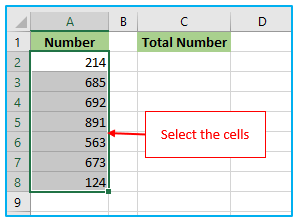
Step 1: Select the range of cells that you want to name dynamically.
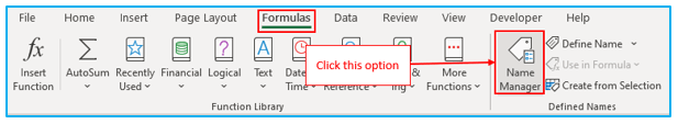
Step 2: Open the “Name Manager” dialog box by clicking on the “Formulas” tab in the ribbon and then clicking on “Name Manager”.
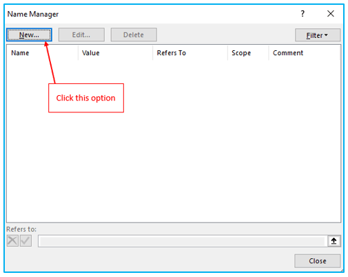
Step 3: In order to establish a new named range, click the “New” button.
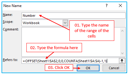
Step 4: In the “Name” field, give your range a name.
In the “Refers to” field, enter the formula that defines your dynamic named range. For example, if you want to create a range that includes all the values in column A from the second row to the last row, you will enter =OFFSET(Sheet1!$A$2,0,0,COUNTA(Sheet1!$A:$A)-1,1)
Click on “OK” to create your named range. Then click “Close” button to close the “Name Manager” dialog box.
A reference to a range that is a given number of rows and columns from a beginning cell or range is returned by the OFFSET function. The following explanations are given for each part of the formula:
reference: The starting point for the range. Since Sheet1’s cell A2 serves as our starting point in this example, we would enter “Sheet1!$A$2” in this section of the formula.
rows: The number of rows to offset from the starting point. In this case, we want to start from row 2, so we would enter “0” in this part of the formula.
cols: The number of columns to offset from the starting point. In this case, we want to start from column A, so we would enter “0” in this part of the formula.
height: The number of rows to include in the range. In this case, we want to include all the rows in column A from the second row to the last row, so we use the COUNTA function to count the number of non-blank cells in column A and subtract 1 to exclude the header row. This part of the formula would look like “COUNTA(Sheet1!$A:$A)-1”.
width: The number of columns to include in the range. In this case, we only want to include one column (column A), so we enter “1” in this part of the formula.
Once you have created your Dynamic Named Range, you can use it in formulas, charts, and other features within Excel, knowing that it will automatically adjust as your data changes.
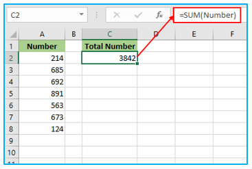
Step 5: Apply the below formula in cell C2
=SUM(Number)
Now, you don’t have to type or select any cell in column A. Just enter the named range “Number”.
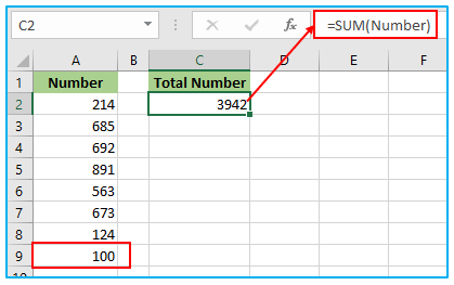
Step 6: Now, Excel automatically updates the sum whenever you add a value to the range.
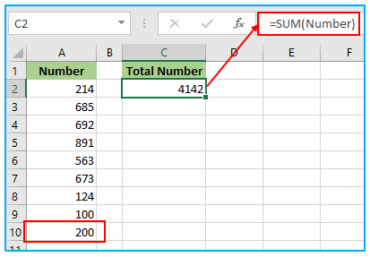
Step 7: After adding a value in cell A10, the result looks like this:
It’s worth noting that there are many different ways to define a dynamic named range in Excel, and the formula used will depend on the specific requirements of your worksheet. However, the basic process of creating a Dynamic Named Range remains the same, as outlined in these steps.
4. Rules for Creating Dynamic Named Range in Excel:
If we keep a few things in mind when we define the names, it will assist. But first, we need to adhere to Microsoft’s predetermined rules, which are listed below.
- The name’s first letter should be followed by a letter, an underscore (_), or a backslash ().
- No gap is allowed between two words.
- As an example, A50, B10, C55, etc., are not acceptable cell references for names.
- Excel employs letters like C, c, R, and r as selection shortcuts, so we are forbidden to use them.
- The term “Define Name” is case-insensitive. MONTHS and months are interchangeable nouns.
For ready-to-use Dashboard Templates:
