Create Cell Reference in Excel to significantly enhance your data management and analytical capabilities. This foundational skill allows for more dynamic spreadsheets, enabling automatic updates and accurate calculations across multiple datasets. By leveraging cell references, you can streamline workflows, improve data accuracy, and create more interactive and responsive reports. Embrace the power of cell referencing to transform your Excel projects into robust, efficient, and interconnected data models, setting the stage for advanced analysis and informed decision-making.
This Tutorial Covers:
- What is a cell address in Excel
- What is a range reference in Excel
- A1 and R1C1 reference styles
- How to make a reference in Excel
- How to change a cell address in a formula
- How to cross reference in Excel
- Refer to a different workbook
- What is a Cell Reference in Excel
- Relative cell reference
- Absolute cell reference
- Mixed cell reference
- How to switch between different reference types
- Circular reference
- 3-D reference
- Structured reference (table reference)
- Named cells and ranges
1. What is a cell address in Excel?
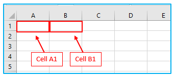
A spreadsheet cell is identified by a cell reference, also known as a cell address, which is made up of a column letter and a row number.
The first cell in column B, for instance, is designated as B1; similarly, the first cell in row 1 is designated as A1, and so forth.
Cell references assist Excel in locating the values the formula should calculate.
For instance, you may use this straightforward formula to copy the value from cell A1 to another cell:
=A1
Use this one to add the values in cells A1 and B1:
=A1+B1
2. What is a range reference in Excel?
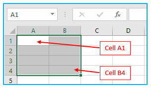
A range in Excel is a group of two or more cells. The address of the upper left cell and the lower right cell, separated by a colon, serve as a range reference.
For instance, the range A1:B4 contains 8 cells, ranging from A1 to B4.
3. A1 and R1C1 reference styles
A1 and R1C1 are the two address styles available in Microsoft Excel.
A1 reference style in Excel:
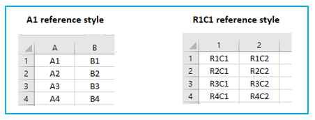
The most frequently used default style is A1. In this design, rows are denoted by numbers and columns by letters, i.e. A1 refers to a cell in row 1, column A.
R1C1 reference style in Excel:
The R1C1 style uses numerals to identify both the rows and columns, i.e. Row 1, column 1, cell indicated by R1C1.
Both the A1 and R1C1 reference styles are demonstrated in the screenshot below:
Click File > Options > Formulas and check the R1C1 reference style box to change the default A1 style to R1C1.
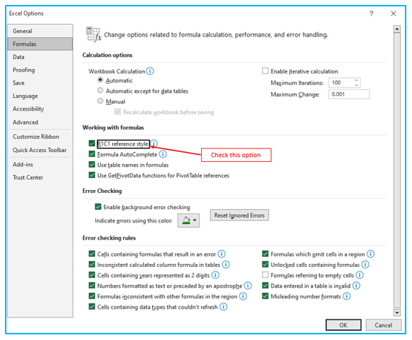
Click File > Options > Formulas and check the R1C1 reference style box to change the default A1 style to R1C1.
4. How to create a reference in Excel?
The procedure of making a reference in Excel:
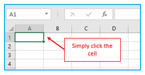
Step 1: To create a formula, simply click the cell you want it in.
Step 2: Choose one of the following:
Directly enter the reference in the cell or formula bar, or select the desired cell by clicking it.
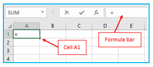
Enter “=” as the equal symbol in the cell or formula bar.
Step 3: To finish the formula, type the final few letters and press the Enter key.
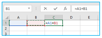
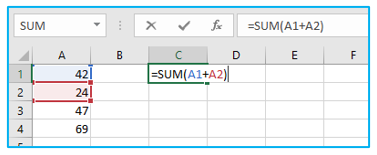
For instance, you would type the equal sign, click cell A1, type the plus sign, click cell B1, and then press Enter to add the numbers in cells A1 and B1:
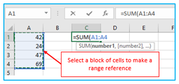
Choose a set of worksheet cells to act as a range reference.
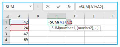
For instance, to sum the values in cells A1, A2, A3, and A4 enter the equal sign, the SUM function’s name, the opening parenthesis, the cells A1 through A4, the closing parenthesis, and press enter key on your keyboard.
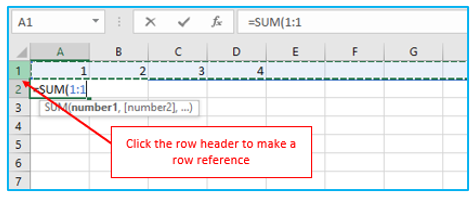
Click the row number or the column letter, accordingly, to refer to the complete row or column.
For instance, begin entering the SUM function to add up all the cells in row 1, and then click the first row’s header to add the row reference to your formula:
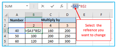
5. How to change a cell address in a formula?
The procedure of changing a cell address or cell reference in a formula:
Step 1: In order to access the Edit mode, either double-click the cell containing the formula or click the cell and press “F2.” This will use a different color to highlight each cell or range that the formula refers to.
Step 2: Any of the following actions will modify a cell address:
- Choose the formula reference, then type a new one.
- Choose a cell or range on the sheet, then choose the reference in the formula.
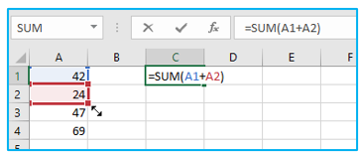
Step 3: Drag the color-coded border of the cell or range to include or exclude more or fewer cells from the reference. Then press Enter key on your keyboard.
6. How to cross-reference in Excel?
You must know not only the target cell or cells but as well as the worksheet and spreadsheet where they are in order to refer to cells in another worksheet or another Excel file. The so-called “external cell reference” can be used for this.
- Refer to a different workbook:
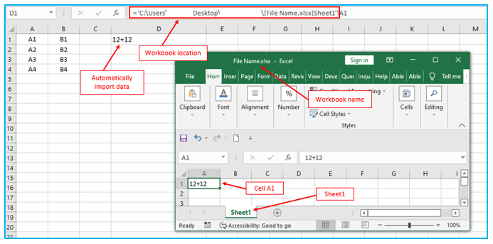
You must place the name of the workbook in square brackets, then the name of the sheet, an exclamation point, and the cell or range address in order to refer to a cell or range of cells in another Excel file. Examples include
=[File Name.xlsx]Sheet1! A1
Be sure to put the path in single quotation marks, for example, if the file or sheet name contains characters other than those in the alphabet.
= ‘[File Name.xlsx]Sheet1’!A1
You don’t have to manually write the path, just like when referencing another sheet. To choose a cell or a group of cells more quickly, turn to the other workbook and do so.
7. What is Cell Reference in Excel?
In Excel, cells make up a spreadsheet. The row value and column value can be used to refer to these cells.
A1 might, for instance, denote the first row (designated as 1) and the first column (specified as A). B3 would be the second column and third row in a similar way.
Excel’s strength comes in its ability to employ these cell references in other cells when formulating data.
There are now three types of cell references available in Excel:
- Relative Cell References
- Absolute Cell References
- Mixed Cell References
You can work with formulas and save time if you are aware of these various cell references (especially when copy-pasting formulas).
- Relative cell reference:
A relative reference is the one without the $ symbol in the row and column coordinates, as A1 or A1:C5. In Excel, all cell addresses are by default relative.
The relative position of rows and columns affects how references are changed when objects are moved or copied across many cells. Therefore, you must utilize relative cell references if you want to perform the same computation repeatedly over multiple columns or rows.
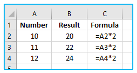
For instance, you would write the following formula in B2 to multiply the integers in column A by 2:
=A2*2
The following formula will be different when transferred from row 2 to row 3:
=A3*2
- Absolute cell reference:
The row or column coordinates with the dollar sign ($) in them, such as $A$1 or $A$1:$C5, are absolute references.
When using the same formula to fill additional cells, an absolute cell reference does not change. Absolute addresses are particularly helpful when you need to copy a formula to other cells without changing references or when you need to do several computations using a value in a single cell.
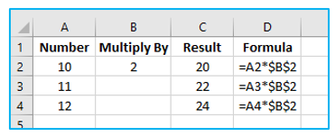
For instance, you would enter the following formula in row 2 to multiply the values in column A by the value in column B2, and then drag the fill handle to replicate the formula down the column:
=A2*$B$2
While the absolute reference ($B$2) will always be locked on the same cell, the relative reference (A2) will change depending on the relative location of the row where the formula is copied:
- Mixed cell reference:
The relative and absolute coordinates $A1 and A$1 are both included in a mixed reference.
There are many circumstances in which only one coordinate, such as a column or row, needs to be fixed.
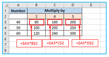
For instance, you might enter the following formula in B3 and then copy it down and to the right to multiply a column of integers (column A) by three separate numbers (B2, C2, and D2):
=$A3*B$2
Because the formula should always multiply the initial numbers in column A, you lock the column coordinate in $A3. The row coordinate must change for other rows; hence it is relative.
By locking the row coordinate in B$2, you may instruct Excel to always choose the multiplier in row 2. Since the multipliers are spread across three different columns, the column coordinate is relative, and the formula should be modified accordingly.
As a result, only one formula is used for all calculations, and it correctly adjusts for each row and column where it is copied:
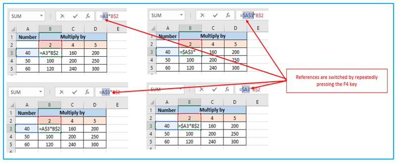
8. How to switch between different reference types?
You can either manually type or delete the $ sign or use the F4 shortcut to go from an absolute reference to a relative reference and vice versa:
The procedure of switching between different reference types:
Step 1: Double-click the cell that the formula is located in and then choose the reference that needs to be updated.
Step 2: To switch between the four reference types, press F4.
The references are switched in the following order by repeatedly pressing the F4 key: A3 > $A$3 > A$3 > $A3.
9. Circular reference
A circular reference is one that, either directly or indirectly, refers back to its own cell.
For instance, if you entered the formula below into cell A1, a circular reference would result:
=A1+250
Circular references are generally a cause of problems; therefore, you should try to limit their use. Furthermore, in some uncommon circumstances, they might be the only option for a particular task.
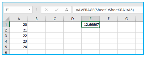
10. 3-D reference:
The term “3-D reference” designates a cell or group of cells that appear on various spreadsheets.
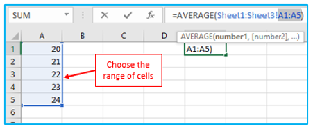
For instance, you may use the AVERAGE function with a 3d reference to get the average of the values in cells A1 through A10 on Sheets 1, 2, and 3:
=AVERAGE(Sheet1:Sheet3!A1:A3)
How to create a formula with a 3D reference is shown below
Step 1: As you would normally, begin entering a formula in a cell by typing =AVERAGE(
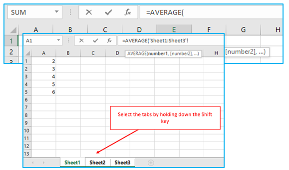
Step 2: To be featured in the 3d reference, click the tab for the first sheet and then click the last sheet’s tab while holding down the Shift key.
Step 3: Choose the cell or range of cells to be calculated in.
Step 4: Once the formula is complete, use the Enter key to finish it.
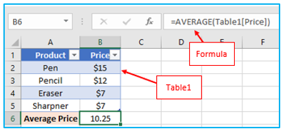
11. Structured reference (table reference)
Instead of using cell addresses in a formula, structured references use table and column names. Only Excel tables’ cells may be used as the subject of such references.
For instance, you can use the following formula to determine the average of the values in Table 1’s “Price” column:
=AVERAGE(Table1[Price])
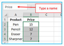
12. Named cells and ranges
In Excel, you may also declare a cell by name or a group of cells by name.
Simply choose the desired cell or cells, enter the desired name in the Name Box, and hit Enter.
You might want to use the defined names instead of the old cell references in your calculations after creating new names.
How to use the defined names instead of the old cell references is shown below
Step 1: Choose the cells that contain the formulas you want to rename the cell references to.
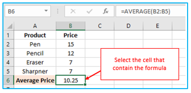
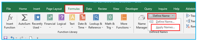
Step 2: Navigate to the “Formulas” tab > “Defined Names” group, select “Define Name” by clicking the arrow next to it, and then select “Apply Names…”
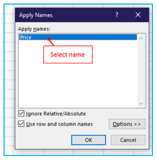
Step 3: Select one or more names in the “Apply Names” dialog box, then click OK.
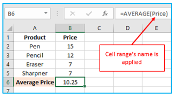
The references in all or particular formulas will then be adjusted to the new names:
Application of Create Cell Reference in Excel
- Formula Linking: Use cell references in formulas to link data across different cells, enabling dynamic calculations that automatically update when the source data changes.
- Data Consolidation: Create cell references to summarize data from multiple sheets or sections within a single worksheet, facilitating organized reporting and analysis.
- Conditional Formatting: Apply cell references in conditional formatting to dynamically format cells based on the value of other cells, enhancing data visualization and emphasis.
- Chart Data Source: Utilize cell references to define the data range for charts, allowing for automatic updates to the chart when the referenced data is modified.
- Data Validation: Implement cell references in data validation rules to ensure consistency and accuracy in user input, based on values in other cells or ranges.
- Dynamic Named Ranges: Use cell references to create dynamic named ranges that automatically adjust as data is added or removed, streamlining data management and lookup operations.
You may be interested:
