This Content Covers:
- What Is an Amortization Schedule?
- Purpose and Benefits of an Amortization Schedule in Excel.
- How to Create an Amortization Schedule using Pre-Built Excel Templates?
- How to Create a Loan Amortization Schedule Manually?
- How to Make a Loan Amortization Schedule with Extra Payments in Excel?
1. What Is an Amortization Schedule?
An amortization schedule is a table or chart that shows the details of each periodic payment made towards a loan or mortgage. It breaks down each payment into its principal and interest components and displays the remaining loan balance after each payment is made.
2. Purpose and Benefits of an Amortization Schedule in Excel.
Purpose: The purpose of an amortization schedule is to provide borrowers with a clear and comprehensive view of their loan payments and to help them understand how much of each payment goes towards paying off the principal amount and how much goes towards paying interest.
Benefits: There are several benefits of creating an amortization schedule. Some of them are given below.
- Clear understanding: Understanding how their loan functions, including how much of their payment goes to interest and how much goes to paying off the loan principle, is beneficial for borrowers.
- Budgeting: By knowing how much their payments would be throughout the course of the loan; borrowers may make the necessary adjustments to their budgets.
- Comparison: It makes it simple to compare several loan possibilities and choose the one that best suits their financial circumstances.
- Transparency: It makes the loan procedure transparent, assisting in avoiding misunderstandings or miscommunication between the borrower and lender.
3. How to Create an Amortization Schedule using Pre-Built Excel Templates?
There are plenty of pre-made Excel templates that you can use to keep track of your loan information. Now let’s see how to create an amortization schedule using Excel templates.
Step 1: Open a worksheet and go to File.
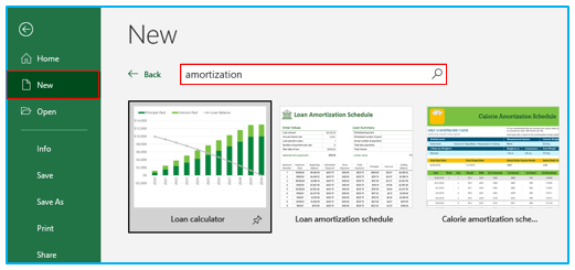
Step 2: Select New and enter the name of the type of amortization table you want to use in the search box.
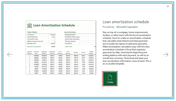
Step 3: If you find your desired template, click on it to see the preview, and select Create option to create this template inside your worksheet.
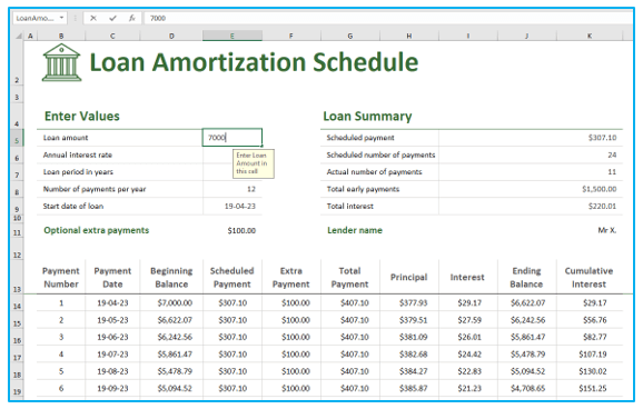
Step 4: Now change the values from the upper section of the table according to your actual loan, interest, and other information. The rest of the table’s data will be generated according to that.
4. How to Create a Loan Amortization Schedule Manually?
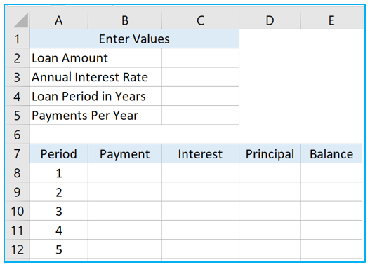
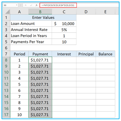
Step 1: To create an amortization schedule manually, first we have to create the structure or the amortization table like this.
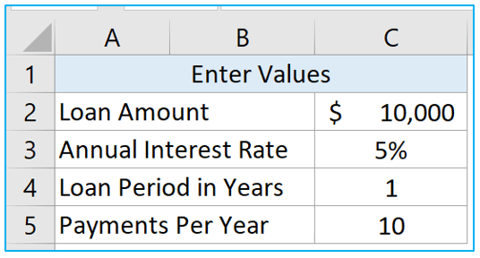
Step 2: Then enter the loan amount, interest rate and other information like the picture below.
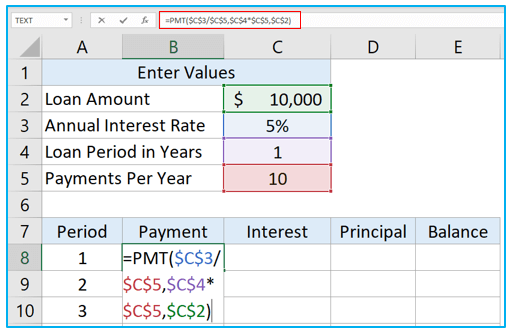
Step 3: Now we have to use the PMT formula to count the payment. Select cell B8 and insert this formula inside the cell.
=PMT($C$3/$C$5,$C$4*$C$5,$C$2)
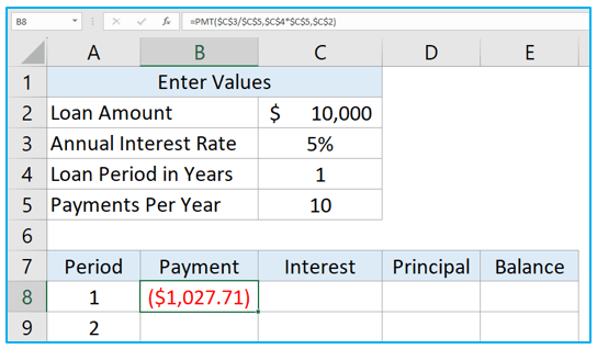
Step 4: Press enter to get first period’s payment. Here we can see that the payment is shown in red color which means this is a negative value. This happened because the loan is paid out of our bank accounts. So, by default, Excel the negative valued in red and enclose them inside parentheses. Follow the next step to get the result as a positive value.
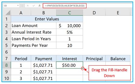
Step 5: To solve this issue we will use a Minus Sign (-) before each of the formulas for payment, interest, and principal. After using a minus sign and converting the result into positive, drag the fill-handle of B8 down to B17 to get all the payment data.
Step 6: Now we will calculate the first period’s interest in cell C8 by using the IPMT formula with a minus sign. Then drag the cell down to C17 to get all the interest data.
=-IPMT($C$3/$C$5,A8,$C$4*$C$5,$C$2)
Step 7: Calculate the principal using the PPMT formula with a minus sign in D8 and drag it downwards.
=-PPMT($C$3/$C$5,A8,$C$4*$C$5,$C$2)
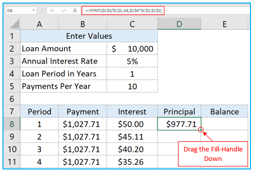
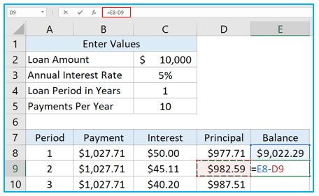
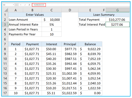
Step 8: We have the payment, interest, and principal data. Now we have to calculate the balance after the first period’s principal payment is paid. To calculate this, select cell E8 and subtract the first period’s principal (D8) from total loan amount (C2).
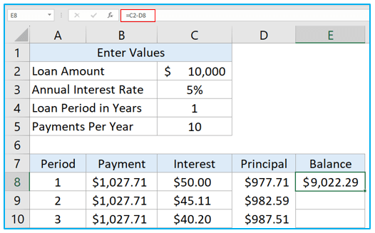
Step 9: Now we have the remaining balance after paying first period’s principal. To calculate the remaining balance after paying second period’s principle in cell E9, we will subtract the second period’s principal (D9) from the remaining balance of E8.
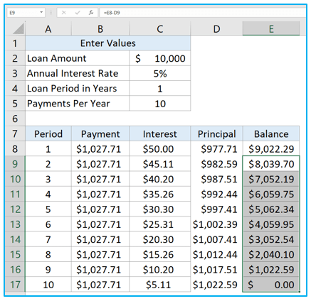
Step 10: Now simply just drag the fill-handle of E9 down to E17. In E17 the balance is $0 which means the loan will be paid by the 10th period with interest.
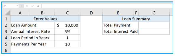
Step 11: Now we will create a Loan Summary section to see how much has to be paid with interest.
Step 12: Select G2 and use the SUM formula to sum the payments and get total payment.
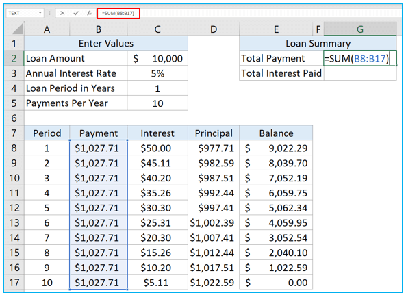
Step 13: Sum the interests to get total interest amount in G3.
5. How to Make a Loan Amortization Schedule with Extra Payments in Excel?
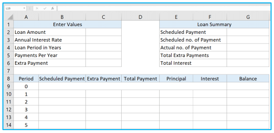
Step 1: First create an amortization table like this. This table will have three parts- enter value, loan summary and the table. If you want to make this table re-usable, make sure to enter the maximum possible number of payment periods. I will use a lower loan amount to explain the whole process so instead of maximum, I’ll create 30 payment periods.
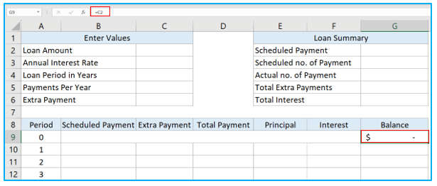
Step 2: If you want you can enter the values like loan amount, interest etc first and then use the formulas or create the table with formulas first then insert the values. Select G9 and link it with C2 (loan amount). So, any amount you enter in the Loan Amount section, will also be updated here for calculation.
=C2
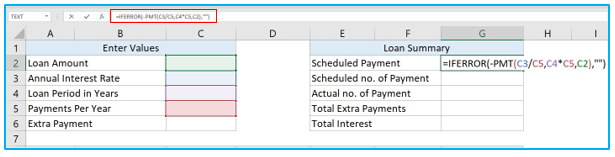
Step 3: Insert the following formula in G2 to get the Scheduled Payment and press Enter.
=IFERROR(-PMT(C3/C5,C4*C5,C2),””)
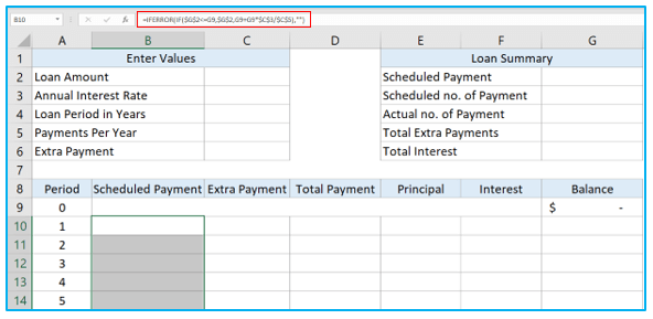
Step 4: Now it’s time to use formulas inside the table to make it usable. Some of the formulas cross-reference which might lead to inaccurate results initially. So, keep inserting the formulas in the table until you enter the very last formula in your amortization table. First insert this formula in B10 and drag it downwards till the last cell of your table. This formula will calculate the scheduled payment.
=IFERROR(IF($G$2<=G9,$G$2,G9+G9*$C$3/$C$5),””)
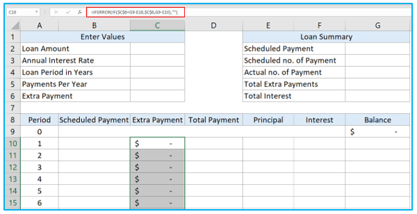
Step 5: Now use this formula in C10 to calculate extra payment. Make sure to drag it till the end for the whole table to work properly.
=IFERROR(IF($C$6<G9-E10,$C$6,G9-E10),””)
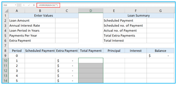
Step 6: This formula will calculate total payments. Insert it in D10, press Enter and drag the cell down.
=IFERROR(B10+C10,””)
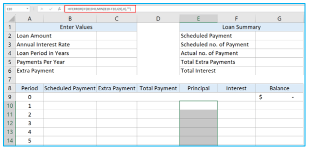
Step 7: To calculate principal, this formula has to be inserted in E10.
=IFERROR(IF(B10>0,MIN(B10-F10,G9),0),””)
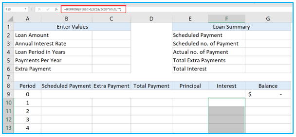
Step 8: Type of paste this following formula in F10 to get interest amount. Drag the fill-handle downwards.
=IFERROR(IF(B10>0,$C$3/$C$5*G9,0),””)
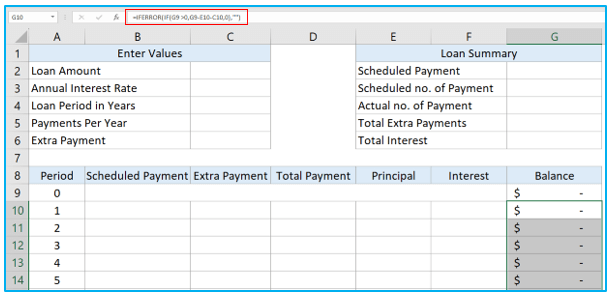
Step 9: Finally insert this inside G10 to calculate the balance and drag to downwards. The amortization table is prepared. Now its time to enter the values.
=IFERROR(IF(G9 >0,G9-E10-C10,0),””)
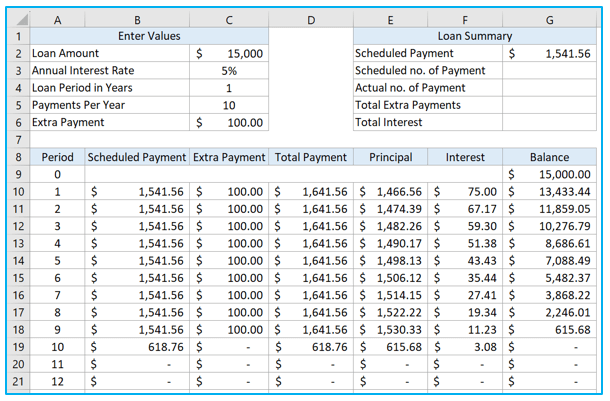
Step 10: Enter the loan amount, interest rate, loan period, payment per year and extra payment values inside the corresponding cells. As soon as you insert the values, the table will return all the data in detail.
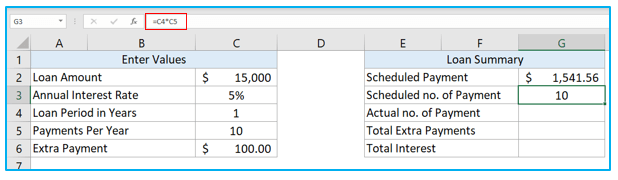
Step 11: Now let’s calculate the Loan Summary. Multiply Loan Period (C4) with Payment per year (C5) to get Scheduled no of payments in G3.
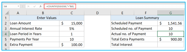
Step 12: Use this COUNTIF formula in G4 to get Actual no of payments.
=COUNTIF(D10:D30,”>”&0)
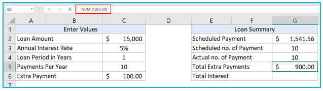
Step 13: Use the SUM function in G5 to get total extra payments.
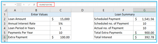
Step 14: Get total interest amount in G6 by using SUM formula.
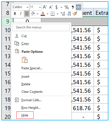
Step 15: Now if you want you can hide the 0 Period row by right clicking on the row and selecting Hide option.
Application of Amortization Schedule in Excel
- Loan Repayment: Generate amortization schedules in Excel to manage loan repayment, detailing principal and interest payments over time.
- Mortgage Planning: Use amortization schedules to plan mortgage payments, optimizing repayment strategies and estimating total interest costs.
- Financial Analysis: Analyze loan terms and repayment scenarios by creating multiple amortization schedules, aiding in financial decision-making.
- Budgeting: Incorporate amortization schedules into budgets to accurately forecast loan payments and ensure financial stability.
- Loan Comparison: Compare different loan options by generating amortization schedules for each, facilitating informed borrowing decisions.
- Investment Evaluation: Assess investment opportunities by analyzing the impact of loan repayments on cash flow using amortization schedules.
For ready-to-use Dashboard Templates:
