Compare Texts of Two Cells in Excel is a fundamental task for data validation, analysis, and manipulation. By utilizing various functions such as IF, EXACT, or conditional formatting, users can easily compare text values in different cells to identify matches, differences, or patterns. Whether you’re reconciling data, detecting duplicates, or verifying consistency in your spreadsheets, mastering the techniques to Compare Texts of Two Cells in Excel is essential for maintaining data accuracy and integrity. Additionally, incorporating advanced methods like string manipulation or regular expressions can further enhance your text comparison capabilities, allowing for more sophisticated analysis and decision-making. With its versatile applications across various industries and functions, knowing how to effectively Compare Texts of Two Cells in Excel equips you with a valuable skill set for efficient data management and analysis.
This Tutorial Covers:
- Compare Text of Two Cells Using “Equal to” Operator
- Compare Two Cells’ Text Using EXACT Function
- Compare Text of Two Cells Using IF Function
- Compare Two Texts by String Length with LEN Function
- Compare Text Strings of Two Cells in Excel by Occurrences of a Specific Character
- Compare Text from Two Cells and Highlight the Matches
- Compare Texts for partial match
- Compare Texts and Find Missing Text Using VLOOKUP
- Find Matches in Any Two Cells in the Same Row
- Find the Unique and Matched Cells by Comparing Their Text
- How to compare multiple cell’s texts
- Formula to compare more than two cells that is not case-sensitive
- Comparing text in many cells using a case-sensitive formula
- How to compare text of one cell with an entire column in Excel
1. Compare Text of Two Cells Using “Equal to” Operator:
Let’s look at a quick formula to compare the text in two cells. The case-sensitive issue won’t be addressed in this instance. The values are the only thing we need to check.
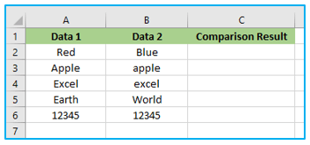
Assume we have the dataset displayed in the following screenshot:

The steps to compare text of two cells using “Equal to” operator are described below:
Step 1: Apply the below formula in cell C2 and you can either copy and paste the formula or drag the formula’s fill handle to the remaining cells.
=A2=B2
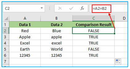
In this example, column A and column B contain pairs of cells that we want to compare. The “Comparison Result” column shows the result of using the “Equal to” operator to compare the text in each pair of cells. The formula =A2=B2 is used in each row to perform the comparison. The result is either TRUE if the text is identical or FALSE if they are different.
Note:
Since this formula does not take into consideration for case-sensitivity, it will display TRUE if the text and values match but do not begin with the same letter.
2. Compare Two Cells’ Text Using EXACT Function:
This section will demonstrate how to use the EXACT function to compare two text cells that will be regarded as an exact match.
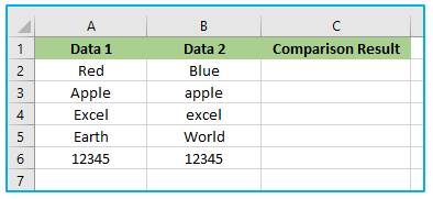
Let’s think about a prior dataset that was used for this procedure.
The steps to compare text of two cells using EXACT Function are described below:
Step 1: Apply the below formula in cell C2 and you can either copy and paste the formula or drag the formula’s fill handle to the remaining cells.
=EXACT(A2,B2)
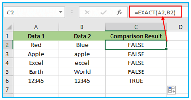
In this example, column A and column B contain pairs of cells that we want to compare using the EXACT function. The “EXACT Comparison Result” column shows the result of using the formula =EXACT(A2, B2) in each row. The function compares the text in each pair of cells and returns TRUE if they are identical (case-sensitive), and FALSE if they are different.
As you can see, the EXACT function accurately distinguishes between uppercase and lowercase letters, providing a precise comparison of text in the cells.
3. Compare Text of Two Cells Using IF Function:
Only the IF function can be used to find matches. Let’s examine the procedure once more using the same dataset. The case-sensitive issue won’t be addressed in this instance.
The steps to compare text of two cells using IF Function are described below:
Step 1: Apply the below formula in cell C2 and you can either copy and paste the formula or drag the formula’s fill handle to the remaining cells.
=IF(A2=B2, “Match”, “No Match”)
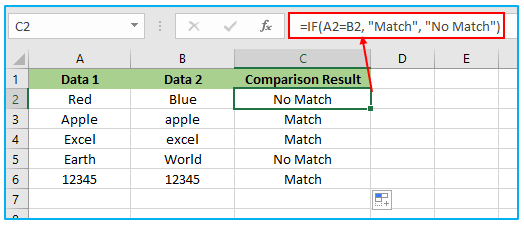
In this example, column A and column B contain pairs of cells that we want to compare using the IF function. The “Comparison Result” column shows the result of using the formula =IF(A2=B2, “Match”, “No Match”) in each row.
The IF function compares the text in each pair of cells (A2 and B2) and returns “Match” if they are identical, and “No Match” if they are different. This provides a clear indication of whether the text in the cells matches or not.
4. Compare Two Texts by String Length with LEN Function:
Let’s examine how we may determine whether or not the text in the two cells has the same string length. The same length text—not the same text—will be the issue.
The length of the string can be the same for two texts with different contents. For instance, despite having the same length, “ABC” and “123” have very distinct meanings. Using only the length of the string to determine equality can result in false positives where there may actually be significant disparities.
We’ll use the same dataset as before.

The steps to compare text of two cells using IF Function are described below:
Step 1: Apply the below formula in cell C2 and you can either copy and paste the formula or drag the formula’s fill handle to the remaining cells.
=IF(LEN(A2)=LEN(B2), “Equal”, “Not Equal”)
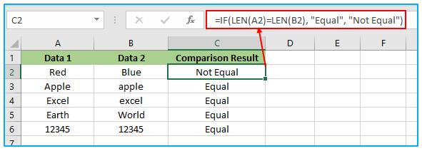
The LEN function in Excel determines the length of a text string. In this case, the formula compares the lengths of the text in cell A2 and cell B2 using the LEN function. If the lengths are equal, the formula returns “Equal”. Otherwise, it returns “Not Equal”.
This method allows you to compare texts based on their string lengths, providing a simple way to determine if they have the same number of characters.
5. Compare Text Strings of Two Cells in Excel by Occurrences of a Specific Character:
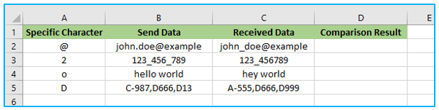
Sometimes it may be necessary to compare cells that contain particular characters. This section will demonstrate how to compare two cells based on the Presence of a Specific Character.
Assume we have the dataset displayed in the following screenshot:
The steps to compare text strings of two cells in excel by occurrences of a specific character are described below:
Step 1: Apply the below formula in cell D2 and you can either copy and paste the formula or drag the formula’s fill handle to the remaining cells.
=IF(LEN(B2)-LEN(SUBSTITUTE(B2, $A2,””))=LEN(C2)-LEN(SUBSTITUTE(C2,$A2,””)),”Same”,”Not Same”)
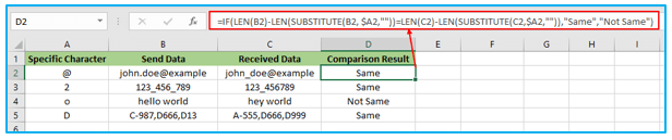
This formula compares the occurrences of a specific character (defined in cell A2) between the text strings in cells B2 and C2. It checks if the differences in length after removing the specific character are equal. If they are equal, it outputs “Same”. Otherwise, it outputs “Not Same”.
6. Compare Text from Two Cells and Highlight the Matches:
We’ll explore how to compare text in this example and highlight any matches.
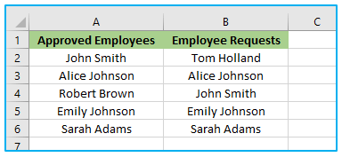
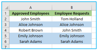
Suppose you have a list of approved employees in one column and another column containing the names of employees who have requested access to a system. You want to check if the employee names requesting access match any of the approved names and highlight the matches.
The steps to compare text from two cells and highlight the matches are described below:
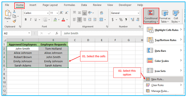
Step 1: Select the range of cells containing both columns, such as A2:B6
Go to the “Home” tab, select “New Rules” option under “Conditional Formatting” in the “Styles” section.
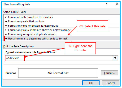
Step 2: Select the rule “Use a formula to determine which cells to format” and type the below formula in the text box of “Format values where this formula is true:”
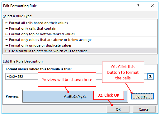
Step 3: After that, choose the formatting style you prefer to highlight the matching cells, like applying a cell background color or font color.
Click “OK” to apply the conditional formatting.
The cells in the “Employee Requests” column that match any of the names in the “Approved Employees” column will be highlighted based on the formatting you selected.
7. Compare Texts for partial match:
Partial matching is something we might consider when comparing two cells. The text of two cells will be partially compared in this section. Excel has many tools that can be used to check parietal components. However, in this instance, we’ll focus on the RIGHT function.
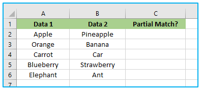
Take a look at this data table to see if the three characters match the two cells serially.
The steps to compare text for partial matches are described below:
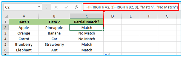
Step 1: Apply the below formula in cell C2 and you can either copy and paste the formula or drag the formula’s fill handle to the remaining cells.
=IF(RIGHT(A2, 3)=RIGHT(B2, 3), “Match”, “No Match”)
The result looks like below:
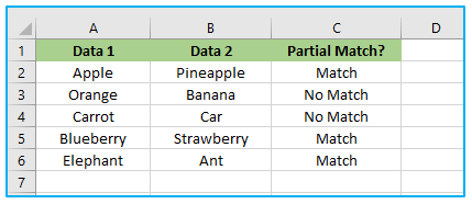
In this illustration, the RIGHT function will be used to compare pairings of text strings in columns A and B. If there is a partial match between the text strings, it is indicated in the “Partial Match?” column.
This formula is used to compare the last 3 characters from the right end of the text strings in cells A2 and B2. If the last 3 characters are the same, the formula returns “Match”. Otherwise, it returns “No Match”.
You can adjust the number in the RIGHT function, depending on how many characters you want to consider to partial match compare.
8. Compare Texts and Find Missing Text Using VLOOKUP:
When you have a list in two columns and want to identify the things or names that are present in one column but not in the other, that is another circumstance in real life where you could need to compare text.
The steps to compare texts and find missing text using VLOOKUP are described below:
Step 1: Apply the below formula in cell C2 and you can either copy and paste the formula or drag the formula’s fill handle to the remaining cells.
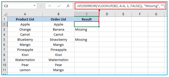
=IF(ISERROR(VLOOKUP(B2, A:A, 1, FALSE)), “Missing”, “”)
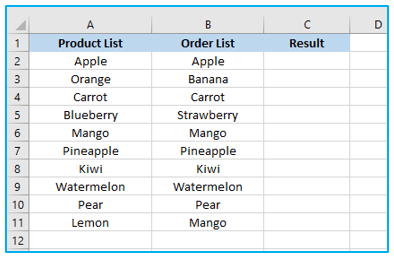
In this example, various products in the “Product List” column and corresponding orders in the “Order List” column. The “Result” column indicates whether the product is missing or not.
This formula is used in the “Result” column. It searches for each product in the “Order List” column (cell B2) within the “Product List” column (range A:A). If a match is not found, it returns an error value, which triggers the ISERROR function. The IF function then checks for the error value and returns “Missing” if there is an error, or an empty string if there is no error.
In the given example, the products “Banana” and “Strawberry” in the “Order List” column are missing from the “Product List” column, as indicated by the “Missing” result. All other products have a match and leave the “Result” column empty.
9. Find Matches in Any Two Cells in the Same Row:
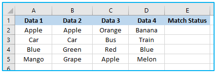
Let’s have a dataset as shown below. Now we will compare the cells with each other, and if we get any two cells matched in the same row, then it will be considered matched.
The steps to find matches in any two cells in the same row are described below:
Step 1: Apply the below formula in cell E2 and you can either copy and paste the formula or drag the formula’s fill handle to the remaining cells.
=IF(COUNTIF(A2:D2, A2)>1, “Match”, “No Match”)
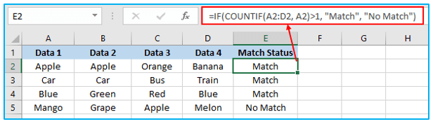
The “Match Status” column will indicate whether there is a match between any two cells in each row. If any two cells in the row have the same value, it will display “Match”. Otherwise, it will display “No Match”.
In this example, the “Match Status” column identifies whether any two cells in each row have matching values. Rows 1, 2, and 3 have matches, while Row 4 does not.
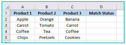
10. Find the Unique and Matched Cells by Comparing Their Text:
Here, our objective is to identify the products that are distinct and that are arranged in a row. We shall consider a match when at least two cells match. It will be deemed a Match if at least two cells match; else, it will be termed Unique.
Assume we have the dataset displayed in the following screenshot:
The steps to find matches in any two cells in the same row are described below:
Step 1: Apply the below formula in cell D2 and you can either copy and paste the formula or drag the formula’s fill handle to the remaining cells.
=IF(COUNTIF(A2:C2, A2)>1, “Match”, “Unique”)
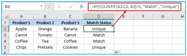
In this example, we have a table with different categories and corresponding products in each row. The “Match Status” column indicates whether the products have a match within the same row.
The “Match Status” column uses the formula =IF(COUNTIF(B2:D2, B2)>1, “Match”, “No Match”) to check if each product appears more than once within its respective row. If a match is found, it displays “Match”; otherwise, it displays “No Match”.
11. How to compare multiple cell’s texts?
Use the formulas covered in the aforementioned examples along with the AND operator to compare more than two cells in a row.
Multiple cell’s texts comparison details are provided in full below.
-
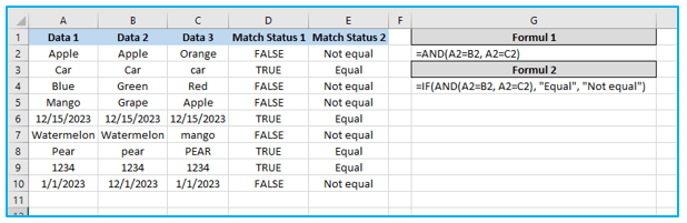
Formula to compare more than two cells that is not case-sensitive:
Use one of the following formulas depending on how you want to present the results:
=AND(A2=B2, A2=C2)
or
=IF(AND(A2=B2, A2=C2), “Equal”, “Not equal”)
If every cell has the same value, the AND formula yields TRUE; otherwise, it returns FALSE. The IF formula returns the labels that you enter, in this case “Equal” and “Not equal.”
The following screenshot shows how the formula flawlessly handles text, dates, and numeric numbers, among other data types:
-
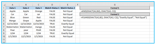
Comparing text in many cells using a case-sensitive formula:
Use the following formulas to check if two or more strings exactly match one another:
=AND(EXACT(A2,B2), EXACT(A2, C2))
Or
=IF(AND(EXACT(A2,B2), EXACT(A2, C2)),”Exactly equal”, “Not equal”)
The first formula provides TRUE and FALSE results, just like in the previous example, but the second formula shows your own texts for matches and differences:
12. How to compare text of one cell with an entire column in Excel?
This dataset has one product list and a cell that matches it. In order to determine the match result, we will now compare the matching cell with the Product Name column.
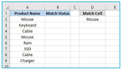
The steps to compare text of one cell with an entire column in Excel are described below:
Step 1: Apply the below formula in cell B2.
=$D$2=A2:A9
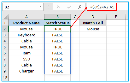
The formula `$D$2=A2:A9` compares the value in cell D2 with each cell in the range A2 to A9. It uses the equality operator (`=`) to check for equality between the values. However, without additional context or an action based on the comparison, it is not possible to determine the intended purpose or outcome of the formula.
In Excel, you can compare strings using functions and techniques to determine equality, partial matches, missing text, and more. Functions like IF, VLOOKUP, MATCH, CONCATENATE, and LEN can be used to perform various types of string comparisons. These comparisons help analyze and manipulate textual data, enabling data-driven decision making and extracting valuable insights from Excel worksheets.
Application of Compare Texts of Two Cells in Excel
- Data Validation: Compare text values of two cells to ensure data consistency and accuracy within a dataset.
- Duplicate Detection: Identify duplicates by comparing text strings in different cells and highlighting matching entries.
- Data Cleansing: Use text comparison to identify and clean inconsistencies or errors in datasets, improving data quality.
- Conditional Formatting: Apply conditional formatting based on text comparison results to visually highlight discrepancies or patterns.
- Case Sensitivity: Compare text values while considering case sensitivity to ensure precise matching and analysis.
- Formula Logic: Utilize text comparison within formulas or functions to automate decision-making processes or calculations in Excel.
You may be interested:
