Compare Columns in Excel allows users to quickly identify differences, spot matches, and detect missing values between two sets of data. By leveraging this feature, users can ensure data accuracy, validate entries, and track changes over time. Whether it’s for error checking or data quality assurance, Compare Columns in Excel is a versatile tool for analyzing and managing data effectively.
This Content Covers:
- Compare two columns in Excel row by row
- Compare two columns for matches or differences in the same row
- Compare two lists for case sensitive matches in the same row
- Compare multiple columns for matches in the same row
- Find matches in all cells in the same row
- Find matches in any two cells in the same row
- Compare two columns and highlight matches
- Compare two columns and highlight matching data
- Compare two columns and highlight mismatches
- Compare two columns and find missing data points
- Compare two columns and pull matching data
- Pull the matching data (Exact)
- Pull the matching data (Partial)
1. Compare two columns in Excel row by row
One of the most frequent jobs while performing data analysis in Excel is comparing the data in each individual row. The following examples show how the IF function can be used to complete this task.
-
Compare two columns for matches or differences in the same row
Procedure of comparing two columns for matches or differences in the same row
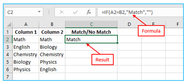
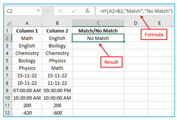
For comparing two columns for matches
Step 1: Write a simple IF formula that compares the first two cells to compare two columns row by row in Excel. On another column in the same row, enter the formula. The formula and result are outlined in Red below.
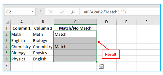
Step 2: After that, to fill all the cells, pull the “Fill Handle” further. The result is outlined in Red below.
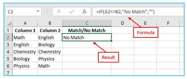
For comparing two columns for differences
Step 1: Write a simple IF formula that compares the first two cells to compare two columns row by row in Excel. On another column in the same row, enter the formula. The formula and result are outlined in Red below.
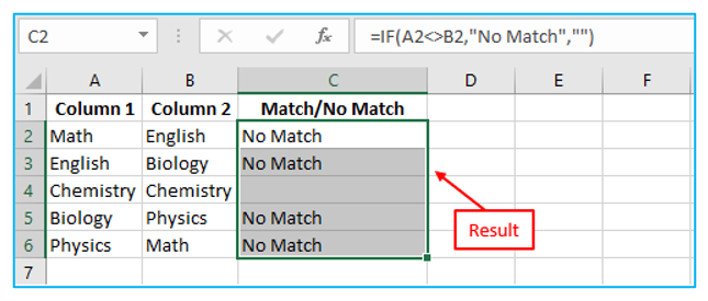
Step 2: After that, to fill all the cells, pull the “Fill Handle” further. The result is outlined in Red below.
For comparing two columns for matches and differences:
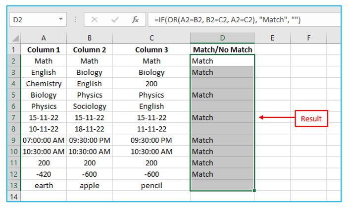
Step 1: Write a simple IF formula that compares the first two cells to compare two columns row by row in Excel. On another column in the same row, enter the formula. The formula and result are outlined in Red below.
Step 2: After that, to fill all the cells, pull the “Fill Handle” further. The result is outlined in Red below.
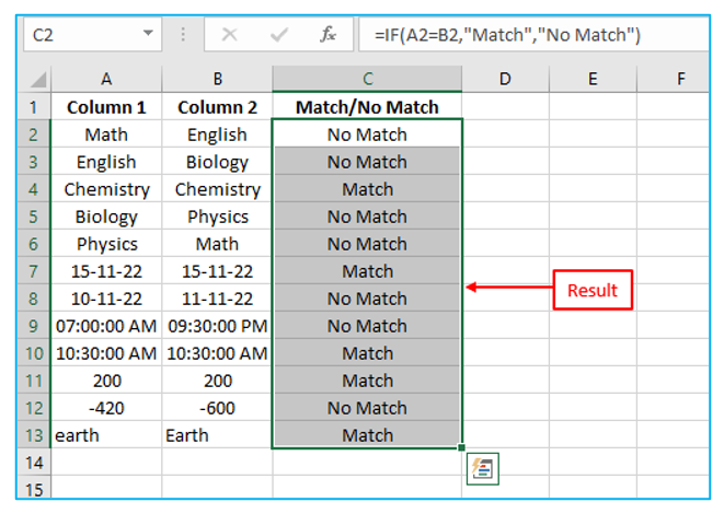
You can see that the formula handles dates, times, numbers, and text strings all equally well.
-
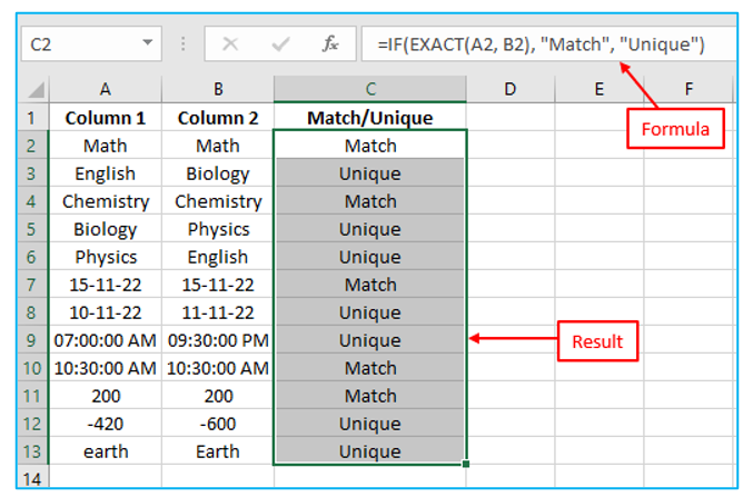
Compare two lists for case sensitive matches in the same row
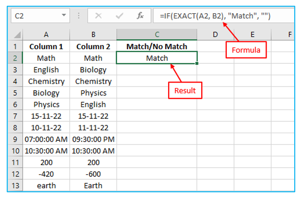
When comparing text values, the simple IF formula disregards case. Use the EXACT function to identify case-sensitive matches between two columns in each row.
Procedure of comparing two lists for case sensitive matches in the same row:
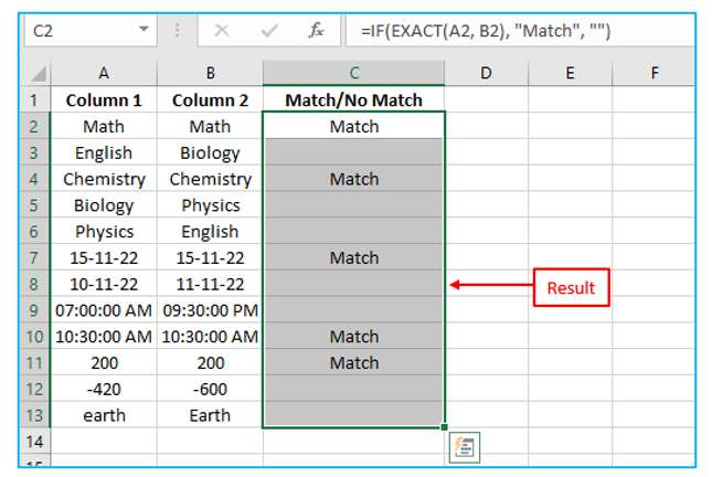
Step 1: Write an EXACT function that compares the first two cells to compare two columns row by row in Excel. On another column in the same row, enter the formula. The formula and result are outlined in Red below.
Step 2: After that, to fill all the cells, pull the “Fill Handle” further. The result is outlined in Red below.
Enter the corresponding text (“Unique” in this example) in the third parameter of the IF function to identify case-sensitive differences in the same row. The formula and result are outlined in Red below.
2. Compare multiple columns for matches in the same row
Multiple columns can be compared in Microsoft Excel using the following standards:
- Find matches in all cells in the same row
- Find matches in any two cells in the same row
-
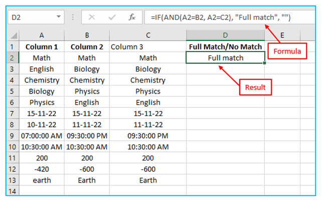
Find matches in all cells in the same row
If there are three or more columns and you want to find rows that have the same values in all cells, an IF formula with an AND statement will work a treat.
Procedure of finding matches in all cells in the same row:
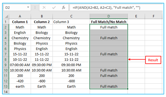
Step 1: Write an IF formula with an AND statement that compares all cells in the same row. On another column in the same row, enter the formula. The formula and result are outlined in Red below.
Step 2: After that, to fill all the cells, pull the “Fill Handle” further. The result is outlined in Red below.
The COUNTIF function would be a more elegant solution if there are many columns:
=IF(COUNTIF ($A2:$E2, $A2)=5, “Full match”, “”)
Where 5 is the number of columns you are comparing.
-
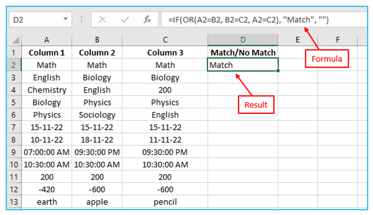
Find matches in any two cells in the same row
Use an IF formula with an OR statement to compare columns for any two or more cells in the same row that have the same values.
Procedure of finding matches in any two cells in the same row:
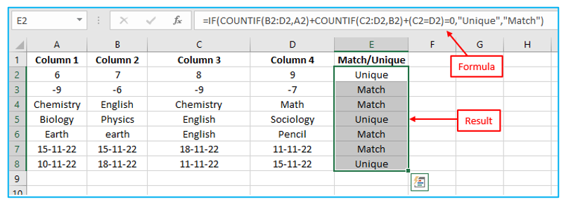
Step 1: Write an IF formula with an OR statement that compares the columns for any two or more cells in the same row that have the same values. On another column in the same row, enter the formula. The formula and result are outlined in Red below.
Step 2: After that, to fill all the cells, pull the “Fill Handle” further. The result is outlined in Red below.
Your OR statement could become overly large if there are several columns to compare. A better option in this situation would be to combine multiple COUNTIF functions. The first COUNTIF counts the number of columns that have the same value as the first column, the second COUNTIF counts the number of columns that have the same value as the second column among the remaining columns, and so on. The formula outputs “Unique” if the count is zero and “Match” in all other cases.
3. Compare two columns and highlight matches
Utilize conditional formatting’s duplication functionality to compare two columns and highlight data that matches.
This is distinct from what we have observed while comparing each row, so take note. We won’t be performing a row-by-row comparison in this example in the case.
-
Compare two columns and highlight matching data
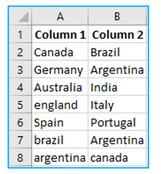
You’ll frequently encounter datasets with matches, even though they might not all be in the same row.
As displayed below
Procedure of highlighting all the matching data:
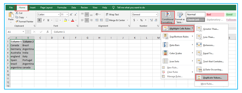
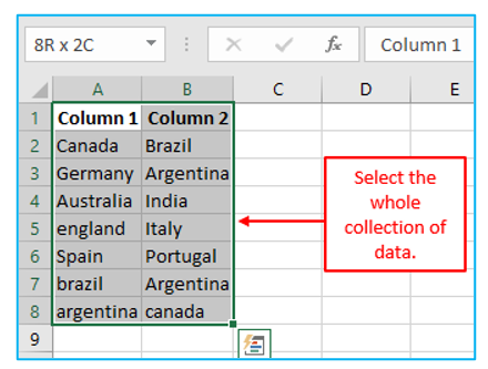
Step 1: Select the whole collection of data, outlined in Red below.
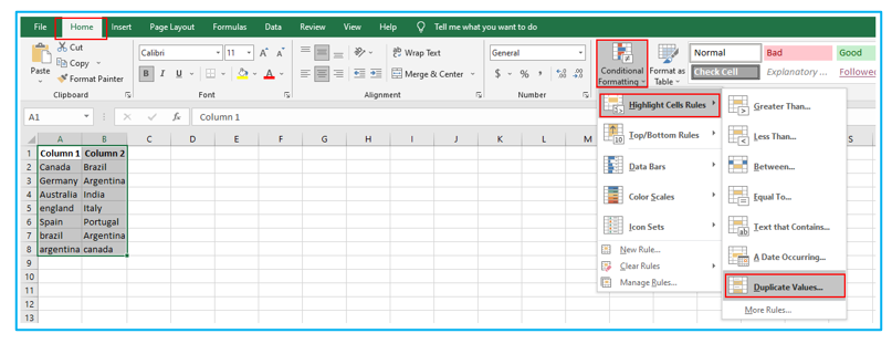
Step 2: Click the “Home” tab, then go to “Styles group”, click on the ‘Conditional Formatting’ option. Then hover the cursor on the “Highlight Cell Rules” option. Click on “Duplicate Values”, outlined in Red below.
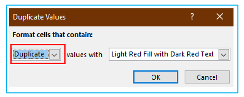
Step 3: Make sure “Duplicate” is chosen in the Duplicate Values dialog box, outlined in Red below.
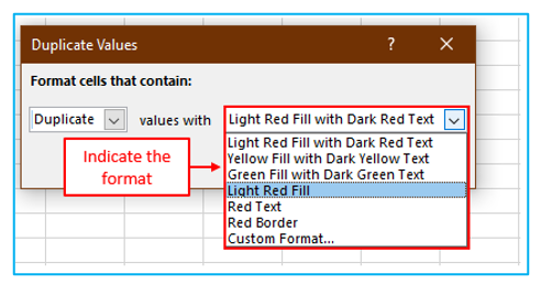
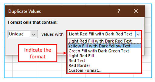
Step 4: Indicate the format and then click ok.
Step 5: After clicking ok, the result looks like below.
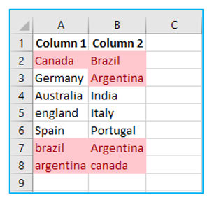
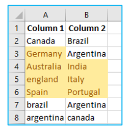
Note that the duplicate rule in conditional formatting is not case-sensitive. As a result, the words “Canada” and “canada” would be marked as duplicates and highlighted.
-
Compare two columns and highlight mismatches
You can also use conditional formatting for this if you want to highlight the names that appear in one list but not the other.
Procedure of highlighting all the mismatching data:
Step 1: Select the whole collection of data, outlined in Red below.
Step 2: Click the “Home” tab, then go to “Styles group”, click on the ‘Conditional Formatting’ option. Then hover the cursor on the “Highlight Cell Rules” option. Click on “Duplicate Values”, outlined in Red below.
Step 3: Make sure “Unique” is chosen in the Duplicate Values dialog box, outlined in Red below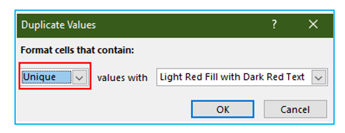
Step 4: Indicate the format and then click ok.
Step 5: After clicking ok, the result looks like below. All the cells with names that are missing from the other list are highlighted.
4. Compare two columns and find missing data points
The lookup formulas must be used if you want to determine whether a data point from one list is present in the other list.
Procedure of Comparing two columns and find missing data points:
Step 1: Write the VLOOKUP formula as below.
=ISERROR(VLOOKUP(A2,$B$2:$B$10,1,0))
After entering the formula, the result is shown as below.
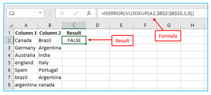
This formula checks whether a country name in column 1 is present in column 2 using the VLOOKUP function. It will return the name from column 2 if it is there; else, it will produce a #N/A error.
These names are the ones that are missing from Column 2 and return the #N/A error.
If the VLOOKUP result contains an error, the ISERROR function would return TRUE; otherwise, it would return FALSE.
Step 2: After that, to fill all the cells, pull the “Fill Handle” further. The result is outlined in Red below.
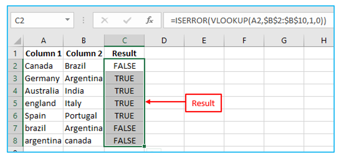
You can filter the result column to retrieve all cells that contain TRUE if you want to receive a list of all the names for which there is no match.
The MATCH function can be used to accomplish the same thing:
=NOT(ISNUMBER(MATCH(A2,$B$2:$B$10,0)))
5. Compare two columns and pull matching data
You need to utilize lookup formulas if you have two datasets and wish to compare items in one list to another in order to get the matching data point.
-
Pull the matching data (Exact)
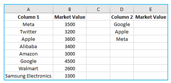
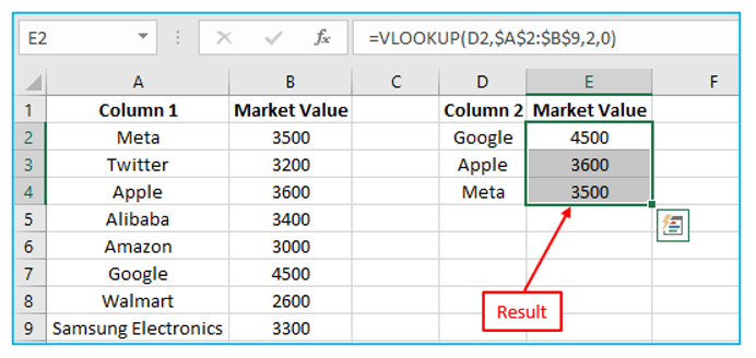
For instance, I want to retrieve the market valuation value for column 2 in the list below. I must first find that value in column 1 before retrieving the corresponding market valuation value.
NOTE: All data are fake and they are using for practice purpose.
Procedure of Comparing two columns and pull matching data (Exact):
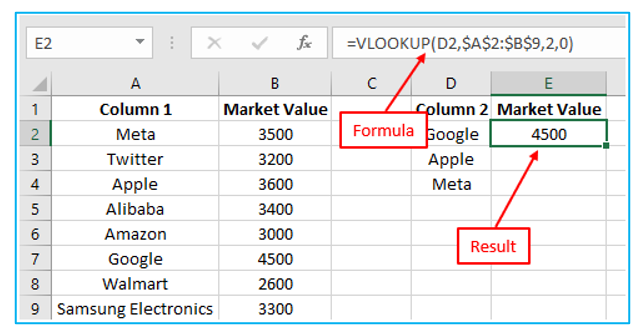
Step 1: Write the VLOOKUP formula as below.
=VLOOKUP(D2,$A$2:$B$9,2,0)
Or,
=INDEX($A$2:$B$9,MATCH(D2,$A$2:$A$9,0),2)
After entering the formula, the result is shown as below, outlined in Red below.
Step 2: After that, to fill all the cells, pull the “Fill Handle” further. The result is outlined in Red below.
-
Pull the matching data (Partial)
Using the lookup formulas above won’t work if you receive a dataset with a slight discrepancy between the names in the two columns.
For these lookup formulas to produce the desired results, an exact match is required.
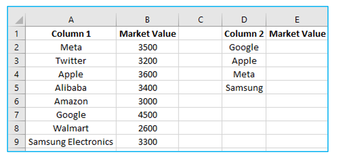
Let’s say you have the data set depicted below. Note that several names in Column 2 are incomplete (such as Samsung instead of Samsung Electronics).
You can use wildcard characters to perform a partial lookup in this situation.
Procedure of Comparing two columns and pull matching data (Partial):
Step 1: Write the VLOOKUP formula as below.
=VLOOKUP(“*”&D2&”*”,$A$2:$B$9,2,0)
Or,
=INDEX($A$2:$B$9,MATCH(“*”&D2&”*”,$A$2:$A$9,0),2)
After entering the formula and after that, to fill all the cells, pull the “Fill Handle” further. The result is shown as below, outlined in Red below.
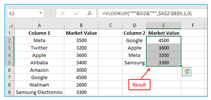
The asterisk (*) in the example above is a wildcard character that can stand in for any number of characters. Any value in Column 1 that also contains the lookup value in Column 2 would be regarded as a match when the lookup value is flanked by it on both sides.
Samsung Electronics, for instance, would match *Samsung* because the symbol * can stand for any number of characters.
Application of Compare Columns in Excel
- Identify Differences: Quickly spot disparities between two columns to ensure data accuracy.
- Highlight Matches: Easily determine matching entries in two separate data sets for validation purposes.
- Detect Missing Values: Instantly locate missing data points or entries between two columns.
- Validate Data Entry: Verify the correctness of entries by comparing them against another column.
- Track Changes Over Time: Monitor changes or updates in data by comparing different versions.
- Error Checking: Use it as a tool for error-checking and data quality assurance in large datasets.
For ready-to-use Dashboard Templates:
