Find circular reference in Excel to troubleshoot and resolve potential errors in your calculations. Circular references can lead to incorrect results and are often hard to spot in complex spreadsheets. This guide aims to equip you with the necessary skills to detect these elusive circular references, ensuring the integrity of your data and the accuracy of your computations. Understanding how to pinpoint and correct circular references is vital for anyone looking to maintain reliable and error-free Excel workbooks.
This Tutorial Covers:
- What is a circular reference in Excel
- How to enable circular references in Excel
- Direct Circular Reference
- Indirect Circular Reference
- How to Use Circular Reference in Excel
- How to find Circular Reference in Excel
- Why is Circular Reference Not Recommended
- Outcomes
- Points to Remember
1. What is a circular reference in Excel?
A circular reference in Excel occurs when a formula in a cell refers to the same cell or depends on another formula that refers back to the original cell, creating a loop that Excel cannot resolve. For example, if cell A1 has a formula “=A1/10”, this creates a circular reference because the formula refers back to the same cell. Similarly, if cell A1 has a formula “=A2” and cell A2 has a formula “=A1”, this also creates a circular reference because the formula in each cell depends on the value of the other cell.
2. How to enable circular references in Excel?
By default, Excel does not allow circular references because they can cause calculation errors and make your spreadsheet unreliable.
However, you can enable circular references in Excel by following these steps:
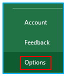
Step 1: Click on the “File” tab, and then select “Options” from the available options to access the “Excel Options” dialog box.
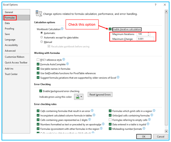
Step 2: In the “Excel Options” dialog box, navigate to the “Formulas” tab by clicking on it.
Locate the “Enable iterative calculation” box in the “Calculation options” section and check it to “Enable iterative calculations”.
In the “Maximum Iterations” box, enter the maximum number of times you want Excel to recalculate the formulas (the default is 100).
In the “Maximum Change” box, enter the maximum amount of change you want to allow between each calculation (the default is 0.001).
Click “OK” to save your changes.
The previous steps would allow Excel to perform iterative calculations.
Also, allow me to briefly describe the two possibilities for the iterative calculation:
Maximum iterations: This is the maximum amount of times Excel should calculate before displaying the result. Therefore, if you enter 100, Excel will execute the loop 100 times before displaying the outcome.
Maximum Change: The calculation would end if this maximum change could not be obtained between iterations. The value is initially set to.001. The outcome would be more accurate the lower this value was.
Keep in mind that Excel needs more time and resources to do an iteration the more times it is performed. If you leave the maximum iterations set high, Excel may become sluggish or even crash.
Note: Excel will no longer display the circular reference warning prompt and will instead display it in the status bar when iterative calculations are enabled.
3. Direct Circular Reference
A direct circular reference in Excel occurs when a formula in a cell refers directly to itself, creating a loop that Excel cannot resolve. Here’s an example of a direct circular reference in a sample table:
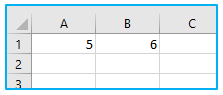
The steps to use direct circular reference are described below:
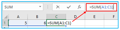
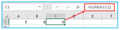
Step 1: Apply the following formula in cell C1:
=SUM(A1:C1)
However, this formula create a direct circular reference because the formula in cell C1 depends on the value of cell C1 creating a loop that Excel cannot resolve.
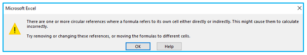
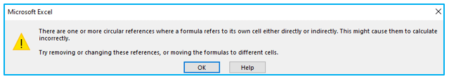
Step 2: After pressing Enter key on your keyboard, the warning with the circular reference error displays. Click OK.
Excel returns a 0 and the result looks like below:
4. Indirect Circular Reference
An indirect circular reference in Excel occurs when a formula in a cell refers to a chain of cells that eventually refer back to the original cell, creating a loop that Excel cannot resolve.
Let’s take a step-by-step look at a basic example.
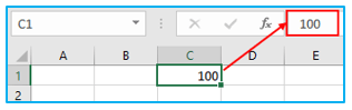
Step 1: Below, in cell C1, enter the number 100.
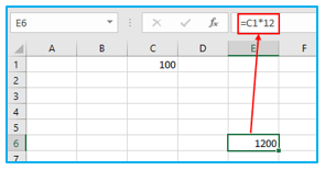
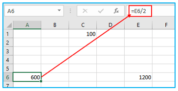
Step 2: Cell C1 is mentioned in cell E6 with multiply by 12.
Step 3: Cell E6 is mentioned in cell A6 and divided by 2.
Step 4: Everything is fine at this time. Now use the following formula to replace the value 100 in cell C1:
=A6*4
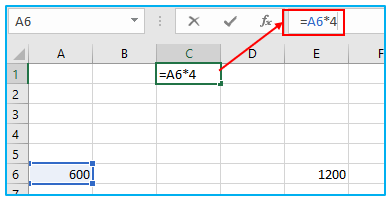
Step 5: Enter the key. An error message with a circular reference occurs. Select OK.
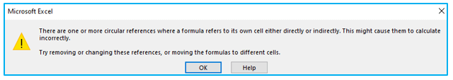
Excel returns a 0 and the result looks like below:
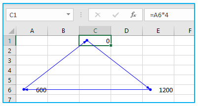
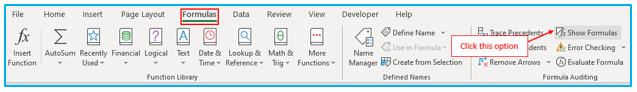
Step 6: On the “Formulas” tab, select “Show Formulas” from the “Formula Auditing” group.
Cell C1 refers to cell A6. Cell A6 refers to cell E6. Cell C1 is referenced in cell E6.
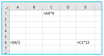
In conclusion, cell C1’s formula makes a subtle reference to itself. It is impossible to do this. In addition, the formulas in cells A6 and E6 provide a circle-shaped reference to their own cells.
5. How to Use Circular Reference in Excel?
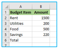
Suppose you have a dataset like the one below:
Here’s a step-by-step guide on how to use circular reference in Excel:
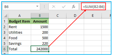
Step 1: In cell B6, type the below formula.
=SUM(B2:B6)
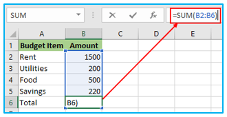
As we enabled iterative calculation, the cell that contained the total value returned 24200 instead of 2420.
6. How to find Circular Reference in Excel?
The steps listed below can be used in Excel to find circular references:
Step 1: In the Excel ribbon, select the “Formulas” tab. To select “Error Checking” in the “Formula Auditing” group, click on the drop-down arrow next to it. From the drop-down box, choose “Circular References”. This displays the most recent circular reference entered. We must then tap on the cell that is displayed under “Circular References.”
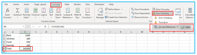
When we carry out this, the status bar notifies us that our workout manual has circular references and identifies which cell it refers to:
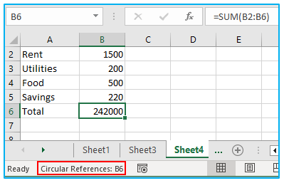
Only the cell reference is displayed if we discover a circular reference in another Excel sheet. As an alternative, it shows a “circular reference.”
After saving, the file displays a warning that one or more of its formulas contain circular references when we reopen it.
7. Why is Circular Reference Not Recommended?
Excel Circular references can lead to a number of problems, including:
- Calculation errors: When a circular reference is present, Excel cannot calculate the result of the formula correctly, which can lead to calculation errors and incorrect results.
- Slow performance: Circular references can cause your spreadsheet to run more slowly and can make it difficult to perform other tasks, such as formatting or data entry.
- Difficulty in auditing and troubleshooting: When a circular reference is present, it can be difficult to track down the source of the problem, as it may involve a chain of cells referencing each other. This can make auditing and troubleshooting the spreadsheet more challenging.
- Maintenance issues: Circular references can make a spreadsheet difficult to maintain, especially if it is shared with other users or if you need to make changes to it over time. Data mistakes and inconsistencies may result from this.
To avoid these issues, it is important to minimize or eliminate circular references in your Excel spreadsheets. If you do need to use circular references, be sure to use them only when necessary and to limit their use to a small number of cells. Additionally, use Excel’s built-in auditing tools to identify and resolve circular references as quickly as possible.
8. Outcomes:
- The arrangement unites, which signifies a steady ultimate product is to come. It is a seductive state.
- The arrangement wanders, suggesting that the difference between the current and previous results increases from cycle to emphasis.
- The configuration alternates between two values. For instance, the result after the first iteration is 1. The outcome is 10 after the next cycle, and 100 after the one after that.
9. Points to Remember:
- Exceed expectations does not appear the notice message over and over when we utilize more than one equation in Exceed expectations with a circular reference.
- While using circular reference, we must always check that iterative computation in the Excel sheet is enabled. Circular references could not be used otherwise.
- The circular reference may lead our function to become repetitious until a specific condition is met, which could slow down our computer.
- To continue with the circular reference, enter the smallest value under the Maximum Change Value field. The more precise the outcome and the longer it will take Excel to calculate a worksheet, the smaller the number.
- After saving, the file displays a warning that one or more of its formulas contain circular references when we reopen it. Therefore, constantly pay attention to the warning and ensure that circular references are enabled.
For ready-to-use Dashboard Templates:
