The CRITBINOM function in Excel is an indispensable tool for critical decision-making and risk assessment. Whether you’re determining safety stock levels, assessing project risks, ensuring quality control, making financial decisions, or analyzing probabilities in gaming scenarios, this function empowers you to find the critical number of successful events needed to meet your objectives. By harnessing the power of CRITBINOM in Excel, you can make informed choices and navigate complex situations with confidence. It’s an essential feature for anyone seeking precision and reliability in their calculations within the Excel environment.
- What is the CRITBINOM Function?
- How to use the CRITBINOM Function in Excel?
- How to calculate Basic CRITBINOM in excel?
- Apply CRITBINOM with Variable Inputs
- Apply CRITBINOM Syntax.
1. What is the CRITBINOM Function?
The CRITBINOM function is used in spreadsheet programs such as Microsoft Excel and Google Sheets to calculate the minimum critical value (the number of successful trials required for a given probability of success) for a binomial distribution. In other words, it helps determine the minimum number of attempts required to achieve a certain level of success in a series of independent binary events (success/failure, yes/no, etc.).
Something you need to remember about CRITBINOM Function
- VALUE! error – Occurs if any of the given arguments are not numbers.
If the test argument is not an integer, it is truncated.
- NUM! error – Occurs when:
The given test argument is less than 0; or
The argument of the given probability is < 0> 1; or
The given alpha argument is <0>1.
2. How to use the CRITBINOM Function in Excel?
There are some rules for using the CRITBINOM Function in Excel. Below is a show of how to use it. You can follow this.
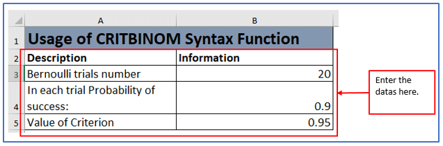
Step 1: So here are some data, which you need while using the CRITBINOM Function in Excel
- Bernoulli trials number: 20
- In each trial Probability of success: 0.9
- Value of Criterion: 0.95
Step 1: First, enter the above data in Excel sheet.
You can see below that all the data are placed in Excel.
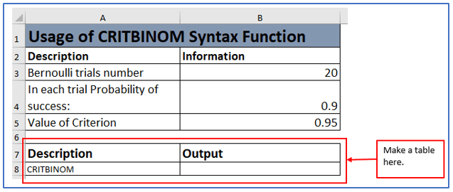
Step 2: Now, make another table to get the CRITBINOM result.
A table has been prepared below.
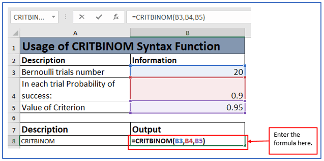
Step 3: Now, use the formula.
The formula for this example will be: =CRITBINOM(B3,B4,B5)
The formula has been placed according to its data.
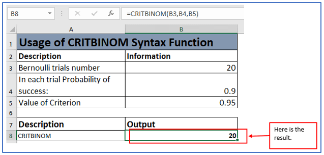
Step 4: After setting the formula, press Enter. Then it will display the answer.
Here is the answer below.
3. How to calculate Basic CRITBINOM in excel?
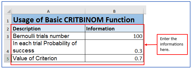
Suppose, while operating an analysis you want to know the minimum number of people you need to interview In each trial Probability of success: is 30% and Value of Criterion is 70% chance of receiving at least one positive response . Bernoulli’s trials number is 100. In the above example, here is calculating and showing the process of Basic CRITBINOM in Excel.
Where,
Bernoulli trials number: 100
In each trial Probability of success: 30% or 0.3
Value of Criterion: 70% or 0.7
Step 1: First, enter the above data in excel sheet.
You can see below that all the data are placed in excel.
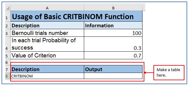
Step 2: Now, make another table to get the CRITBINOM result.
A table has been prepared below.
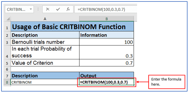
Step 3: Now, use the formula.
In the Basic CRITBINOM the formula is: =CRITBINOM(100,0.3,0.7)
The formula has been placed according to its data.
Step 4: After entering the formula, press Enter. Then it will display the answer.
Here is the answer below.
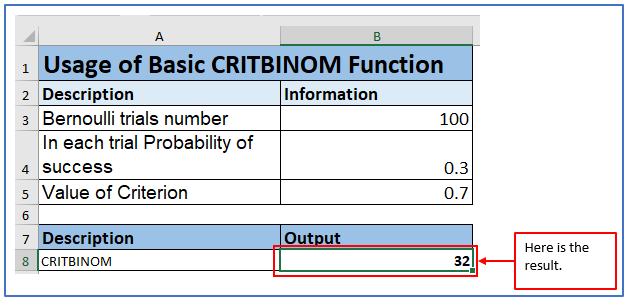
Here you can see that the value is 32. In this circumstance, you need to survey 32 people to have a 70% chance of getting at least one positive response.
4. Apply CRITBINOM with Variable Inputs
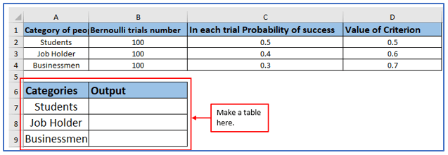
Here, suppose you have to survey with different categories of people and the number of attempts will be in this case the data will be in cell A1, the probability of success in cell B1, and the criterion value in cell C1. Here is an example:
For the Student survey,
- Bernoulli trials number: 100
- In each trial Probability of success: 50%
- Value of Criterion: 50%
For the Job holder survey,
- Bernoulli trials number: 100
- In each trial Probability of success:40 %
- Value of Criterion: 60%
For the Businessmen survey,
- Bernoulli trials number: 100
- In each trial Probability of success: 30 %
- Value of Criterion: 70%
Step 1: Entering the above data in an excel sheet and you can follow it.
You can see below, All the data are placed in excel.

Step 2: Now, make another table to get the result of every categories.
A table has been prepared below.
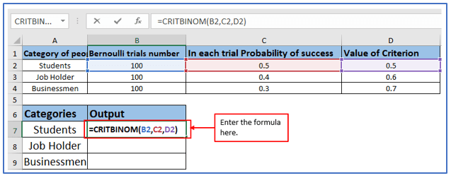
Step 3: Now, use the formula.
The formula will be: =CRITBINOM(B2,C2,D2)
The formula has been placed according to its data.
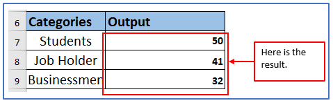
Step 4: After setting the formula, press Enter. Then it will display the answer.
Here is the answer below.

Step 5: Use the same formula for Businessmen and job holders.
For job holders the formula will be: =CRITBINOM(B3,C3,D3)
For Businessmen the formula will be: =CRITBINOM(B4,C4,D4)
Here is the result of every categories of people from the survey:
5. Apply CRITBINOM Syntax.
This function takes inputs such as probability of success, number of trials, and desired probability threshold, and returns the smallest integer value for which the probability of success is greater than or equal to the specified threshold.
This works is based on three main arguments:
- Probability of success: This is the probability of success in one try. It is a value between 0 and 1, with 0 representing impossible success and 1 representing certain success.
- Number of Attempts (Trials): This is the total number of independent trials or trials.
- Desired Probability Threshold: This is the probability threshold that must be met or exceeded for success.
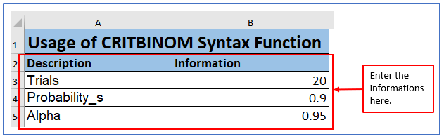
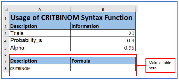
Here is a example for Applying CRITBINOM Syntax. Where,
Bernoulli trials number: 20
In each trial Probability of success: 0.9
Value of Criterion: 0.95
Step 1: Enter the above data in excel sheet.
Here all the data are seated in excel.
Step 2: Now, make another table to get the result of CRITBINOM Syntax.
A table has been prepared below.
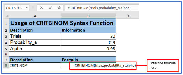
Step 3: For CRITBINOM Syntax the formula will be:
=CRITBINOM (trials,probability_s,alpha)
The formula is using in this picture.
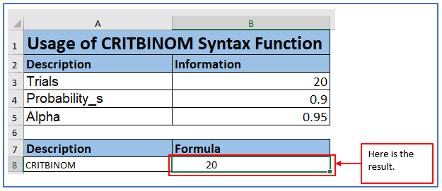
Step 4: After using the formula, here is the answer below.
Application of CRITBINOM function in Excel
- Calculate Critical Value for a Specific Number of Successes:
- Use CRITBINOM to find the smallest number of successful trials required to reach a desired probability of success.
- Determine Safety Stock Levels:
- Estimate the minimum inventory level needed to ensure a certain service level, considering demand and lead time variability.
- Risk Assessment in Project Management:
- Evaluate project risks by identifying the minimum number of successful events needed for a project to succeed.
- Quality Control in Manufacturing:
- Determine the minimum number of defective items that must be found in a sample to reject a batch based on quality standards.
- Financial Decision-Making:
- Assess the probability of a specific number of profitable investments or events occurring in a given financial portfolio.
- Gaming and Probability Analysis:
- Analyze games of chance or probability-based scenarios by calculating the critical number of successful outcomes.
The CRITBINOM function is a valuable tool for decision-making and risk assessment across various fields.
You may be interested:
