T.TEST in Excel is a powerful statistical tool used for hypothesis testing. By analyzing sample data, T.TEST helps determine if there’s a significant difference between two sets of data. Whether you’re comparing means, identifying variations, or testing hypotheses, T.TEST provides valuable insights into the reliability of your data. With its straightforward implementation and robust functionality, T.TEST simplifies complex statistical analysis, making it accessible to Excel users of all levels. Whether you’re a student, researcher, or professional analyst, mastering T.TEST can enhance your ability to draw accurate conclusions from your data, ultimately leading to more informed decision-making processes. Unlock the full potential of your data analysis with T.TEST in Excel.
This Tutorial Covers:
- What is T.TEST Function
- Syntax of T.TEST Function
- Arguments of T.TEST Function
- How to use T.TEST Function in Excel
- How to use T.TEST using Analysis Tool Pack
- Things to Remember
1. What is T.TEST Function?
Excel’s T-Test function is used to determine whether one or both of two data sets are part of the same population with the same mean in order to determine the likelihood that there will be a significant difference between them. T-Test, which also considers whether the data sets we are utilizing for calculation are a one-tail or two-tail distribution with a potential equal or potential unequal variance.
-
Syntax of T.TEST Function:
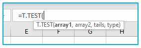
The syntax for the T.TEST function is as follows:
=T.TEST(array1, array2, tails, type)
-
Arguments of T.TEST Function:
The following argument is used by the Excel T.TEST function:
array1: The first data set or range of values for which you want to perform the T-Test.
array2: The second data set or range of values for which you want to perform the T-Test.
tails: Specifies the number of distribution tails to be used in the T-Test. This can be either 1 or 2, representing a one-tailed or two-tailed distribution, respectively.
type: Specifies the type of T-Test to be performed. This can be either 1, 2, or 3, representing a paired test, two-sample equal variance test, or two-sample unequal variance test, respectively.
It’s important to note that the arrays or data sets used in the T-Test function must be of equal size and arranged in a vertical or horizontal layout. Additionally, the T-Test assumes that the data sets are normally distributed and have equal variances, so it may not be suitable for certain types of data.
2. How to use T.TEST Function in Excel?
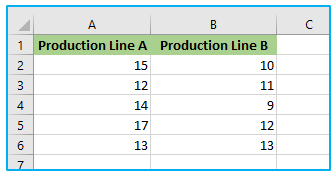
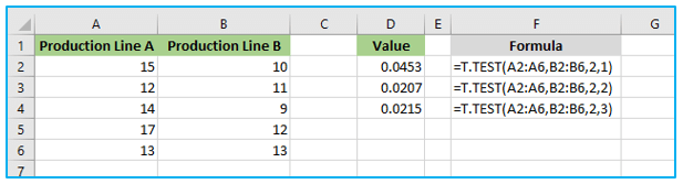
Suppose you work for a company that manufactures widgets. You have two production lines, A and B, and you want to determine whether there is a significant difference in the number of defects between the two lines. You collect data on the number of defects for each line over a period of one month, as shown in the table below:
The steps to use T.TEST formula in Excel are described below:
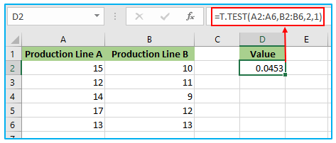
Step 1: Apply the below formula in Cell D2. This test is a type of Paired.
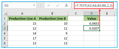
Step 2: Apply the below formula in Cell D3. This test is a type of Two Samples equal variance.
Step 3: Apply the below formula in Cell D4. This test is a type of Two Sample unequal variance.
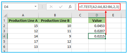
In most cases, the returning result is referred to as the P-value. We can determine that the means of the two sets of data are different if the P-value is less than 0.05. Otherwise, there is no real difference between the two means.
3. How to use T.TEST using Analysis Tool Pack?
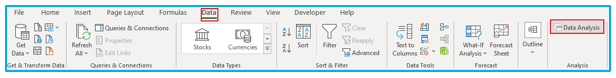
Utilizing the analytical tool set found under the “Data” ribbon tab, we can run the T.TEST.
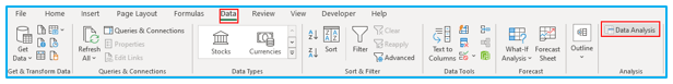
Follow the instructions below to make this option visible if you can’t find it in your Excel file:
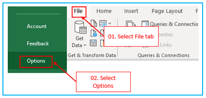
Step 1: Click “Options” after switching to the “File” tab.
Step 2: Click on “Add-Ins”, then select “Excel Add-ins” and then click “Go”.
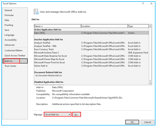
Step 3: Click OK after selecting “Analysis ToolPak”.
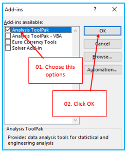
The “Data Analysis” Option must have been enabled as a result.
Suppose you have a dataset like the one below from an earlier section.
The steps to use T.TEST using Analysis Tool Pack in Excel are described below:
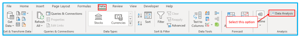
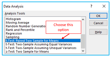
Step 1: Under the “Data” tab, select “Data Analysis”.
Step 2: To find the t-Test, scroll below. Select the first t-Test.
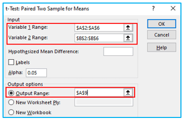
Step 3: After selecting the first t-test, the dialogue box below will appear.
Choose the Output Range, Variable 1 Range, and Variable 2 Range.
Click the OK button after filling out all the boxes.
It will display a thorough report.
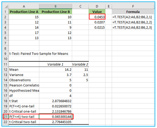
This will provide each data set’s mean, variance, number of observations considered, correlation, and P-value.
We must look at the P-value, which is 0.045300143954446 and significantly lower than the predicted P-value of 0.05 (refer to B21).
Our data are significant if the P-value is less than 0.05.
4. Things to Remember:
- Anything other than numerical numbers is not accepted by the Excel T.TEST formula, therefore we obtain the #VALUE result.
- We will receive #NUM if the tails value is not 1 or 2! error
- To better grasp it, become familiar with the distinction between the One-tailed and Two-tailed tests.
- One of the presumptions is that samples were chosen at random from the enormous amount of data.
- The typical P-value is 0.05, or 5%. Your data are significant if the variance is less than 5%.
Application of T.TEST in Excel
- Comparing Means: T.TEST helps compare the means of two samples to determine if they are significantly different from each other. This is useful in various scenarios, such as comparing the effectiveness of two marketing strategies or the performance of two products.
- Hypothesis Testing: It is commonly used to test hypotheses about the mean of a population based on sample data. For example, you can use T.TEST to determine if a new manufacturing process has significantly improved product quality.
- Quality Control: T.TEST can be employed in quality control processes to assess whether changes in production methods have resulted in statistically significant improvements or deteriorations in product quality.
- Experimental Research: Researchers often use T.TEST to analyze experimental data and determine if the observed differences between groups are statistically significant, helping to validate research findings.
- Biological and Medical Studies: In biological and medical studies, T.TEST is utilized to compare the effectiveness of different treatments or interventions, aiding in evidence-based decision-making in healthcare.
- Educational Assessment: T.TEST can be applied in educational assessment to evaluate the effectiveness of teaching methods or interventions by comparing the academic performance of students before and after implementation.
For ready-to-use Dashboard Templates:
