How to use CHITEST function in excel?

CHITEST function in Excel is a powerful statistical tool that helps validate hypotheses by comparing expected and actual data distributions. By incorporating the CHITEST function in your spreadsheets, you can streamline statistical analysis and make data-driven decisions more confidently. Whether you’re working on research, quality control, or financial forecasting, mastering the CHITEST function enhances the precision and professionalism of your Excel reports.

What Is the CHITEST Function in Excel?
When to Use CHITEST in Excel?
Syntax of in Excel.
How to use CHITEST function in excel? Example-1
How to use CHITEST function in excel? Example-2
What are the Common Errors while using CHITEST Function in Excel?

1. What Is the CHITEST Function in Excel?

The Microsoft Excel CHITEST function returns a value from a Chi Square distribution. The CHITEST function is an integrated function in Excel and is classified as a statistical function Can be used as a worksheet function (WS) in Excel. As a worksheet function, the CHITEST function can be entered as part of the formula in a worksheet cell. By using the CHITEST function in Excel, the probability of observing a particular data record is determined by whether the null hypothesis is true or not.

It helps you understand whether the distribution of data expects a predicted distribution that is often used in hypothesis tests. The CHITEST function helps you determine the likelihood that a cube will achieve this result when it is actually fair. The function returns test statistics for the chi-square distribution. This is a measure of the expected amount of observed data Values that are too close to the observed and expected data indicate an exact matching, whereas those that have a significant difference do not.

2. When to Use CHITEST in Excel?

Once you know what CHITEST is doing, let’s talk about when it can be used. This is primarily used for statistical hypothesis tests, especially categorical data These are some cases where CHITEST can be of great use.

Note Test: Determine if the sample matches the population
Test Independence: Ensures that two categorical variables exist independently of each other.
Comparison of distributions:A comparison of the distribution. The expected distribution is reflected in observation data.

Practically, if you want to address categorical data and test assumptions via distribution, CHITEST is the point of contact Imagine.

3. Syntax of in Excel.

It’s important to follow the Chitest syntax correctly, even though it may seem simple.

CHITEST(actual_range, expected_range)

actual_range: This is the area of observation data representing the collected count or frequency.

expected_range: This is the area of predicted data determined based on a hypothesis or theoretical model.

Both areas must have the same measure If the real data comes from some 3×3 network, then it should be available as well. It is important to make sure this is not possible.

4. How to use CHITEST function in excel? Example-1

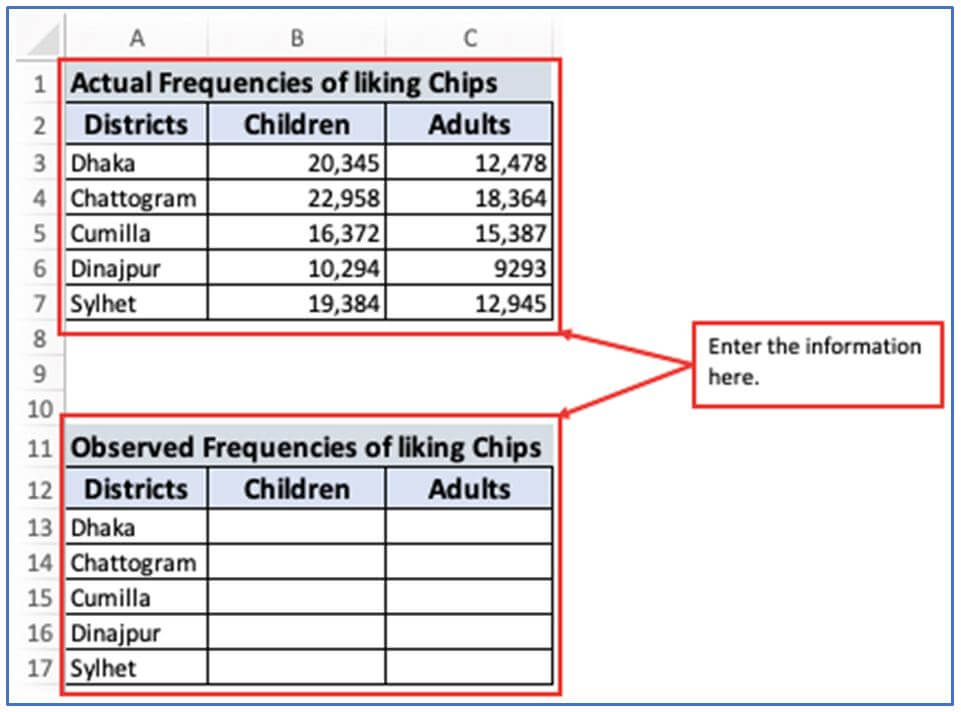
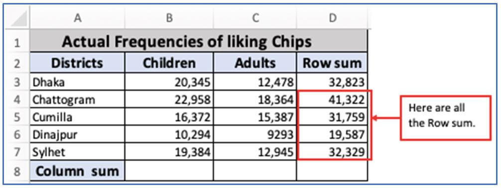
Step 1: Here using two tables to determine the actual and expected frequency of liking Chips in Children and adults in different districts follow the sample data set as an example below.

Entering the data here.

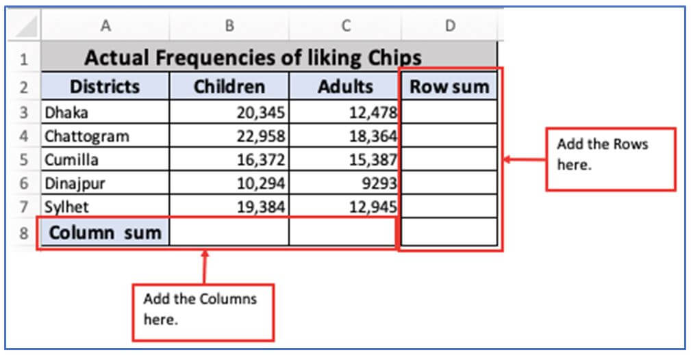
Step 2: Now, add other Rows in D1:D8 to calculate the row sum and add other columns in A8:C8 to calculate the Column sum there.

The columns and rows have been added underneath.

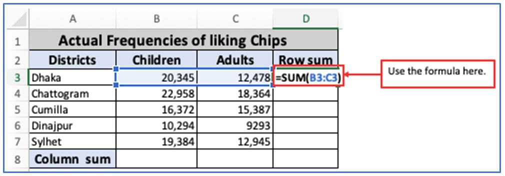
Step 3: For calculating row sum of B3 and C3 use the sum formula in D3. The formula is: =SUM(B3:C3)

Applying the formula below.

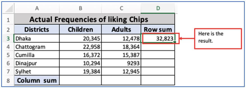
Step 4: After applying the formula press Enter then you will get the result.

Here is the Result.

Step 5: Now apply the same formula for every Excel Rows (D4:D7) or drag down the cursor (+)sign from column D3.

The Actual Frequencies of liking Chips sum of each row is shown.

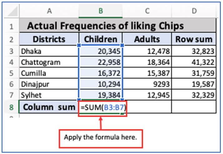
Step 6: Now, for calculating column sum use this formula in B8. The formula: =SUM(B3:B7)

The formula has been operating here.

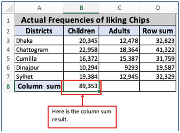
Step 7: Afterwards entering the formula press Enter button.

Here is the column sum result of B8 is 89,353.

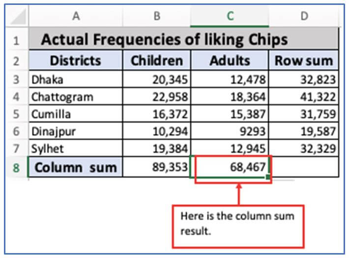
Step 8: Now, use them same formula as shown in B8 or drag them cursor from B8:C8.

Here is them C3:C7 column sum.

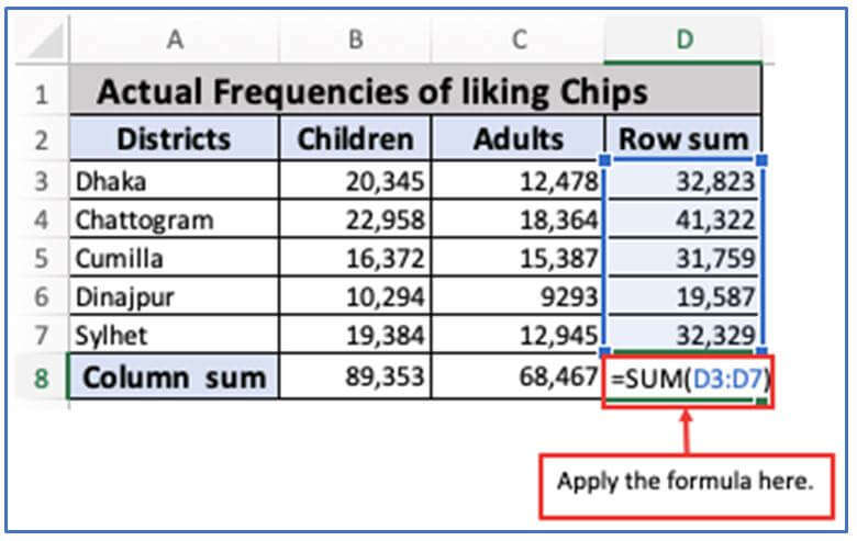
Step 9: You can use the formula for D8: =SUM(D3:D7) or =SUM(B8:C8) in the D8 cell.

=SUM(D3:D7) formula is using here.

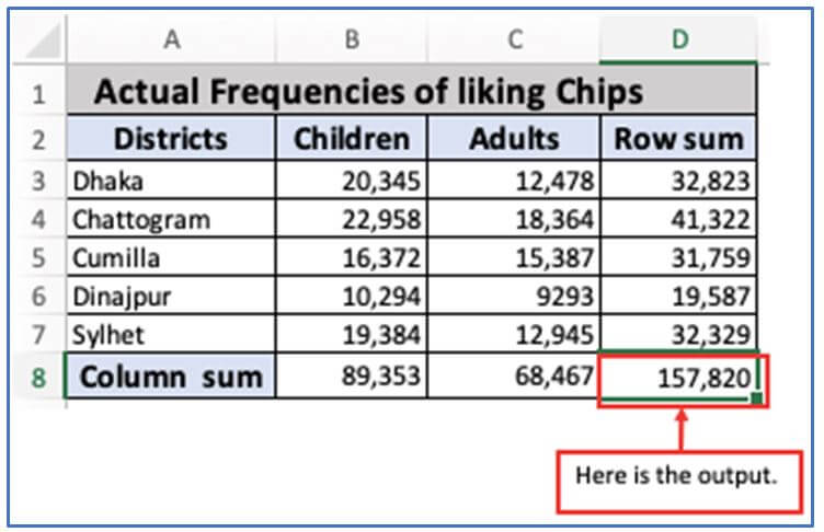
Step 10: Press the input key. Both of these formulas yield the same outcome.

Here is them output.

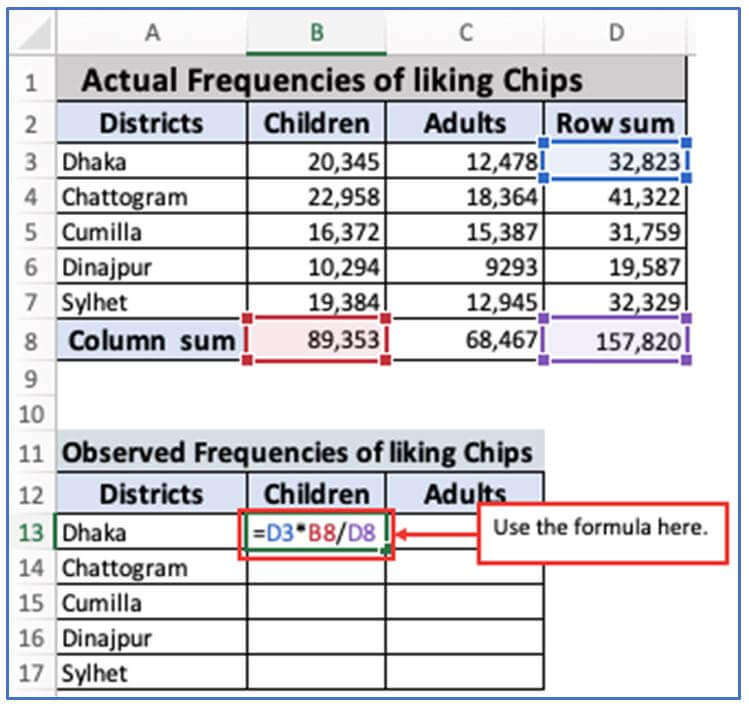
Step 11: To determine the frequencies of each individual cell, you can use this formula: Row Sum*Column Sum/Total

In the B13 cell, input this formula: =D3*B8/D8 as appears below.

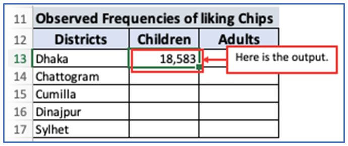
Step 12: Now, press enter and the Observed Frequencies of liking chips of cell B13 result will come out.

Here is the result.

Step 13: Here you can use the the same formula from Step 11 but changing with them cell number from B13:B17. Here are all them formulas:

=D4*B8/D8

=D5*B8/D8

=D6*B8/D8

=D7*B8/D8

Here are the results of B column.

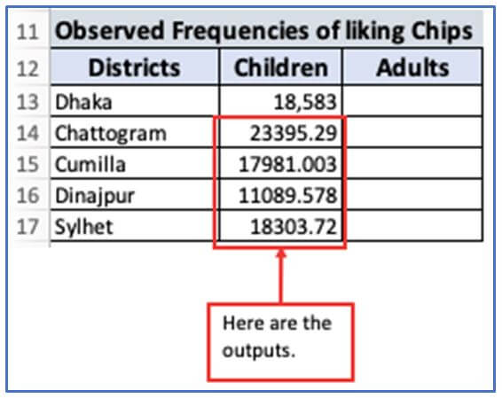
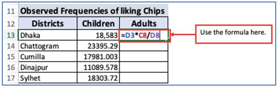
Step 14: For Observed Frequencies of liking chips of Adults enter this formula in cell C13: =D3*C8/D8

Entering them formula here you can see.

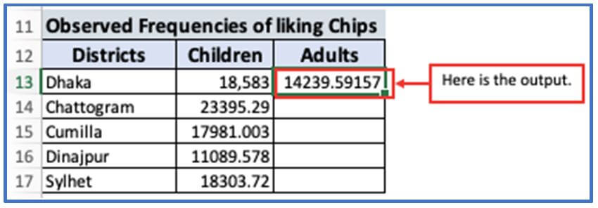
Step 15: Tap on enter button.

Here is the output.

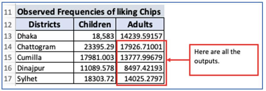
Step 16: You can use the same formula from Step 14 but changing with them cell number from C13:C17. Here are all them formulas:

=D4*C8/D8

=D5*C8/D8

=D6*C8/D8

=D7*C8/D8

Here are the results of B column.

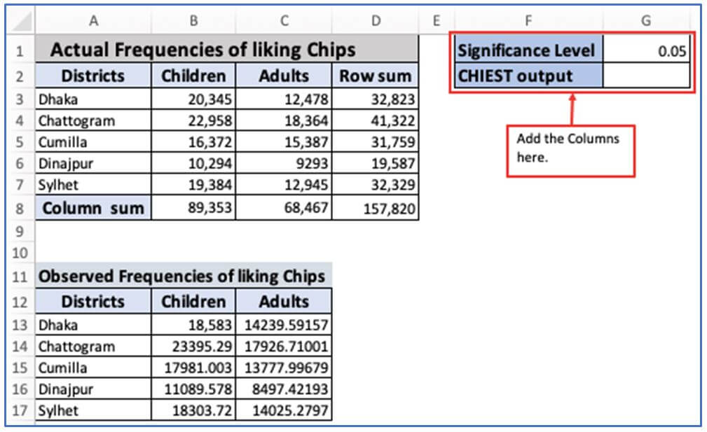
Step 17: The difference between the expected and actual ranges of data sets is not significant when the CHIEST function produces a zero value. Figures from screenshots reveal that the frequencies of Children and the Adults observed have been adjusted for different states. Now, add other columns to enter the Significance Level and to get the result of CHIEST function.

Adding the columns here.

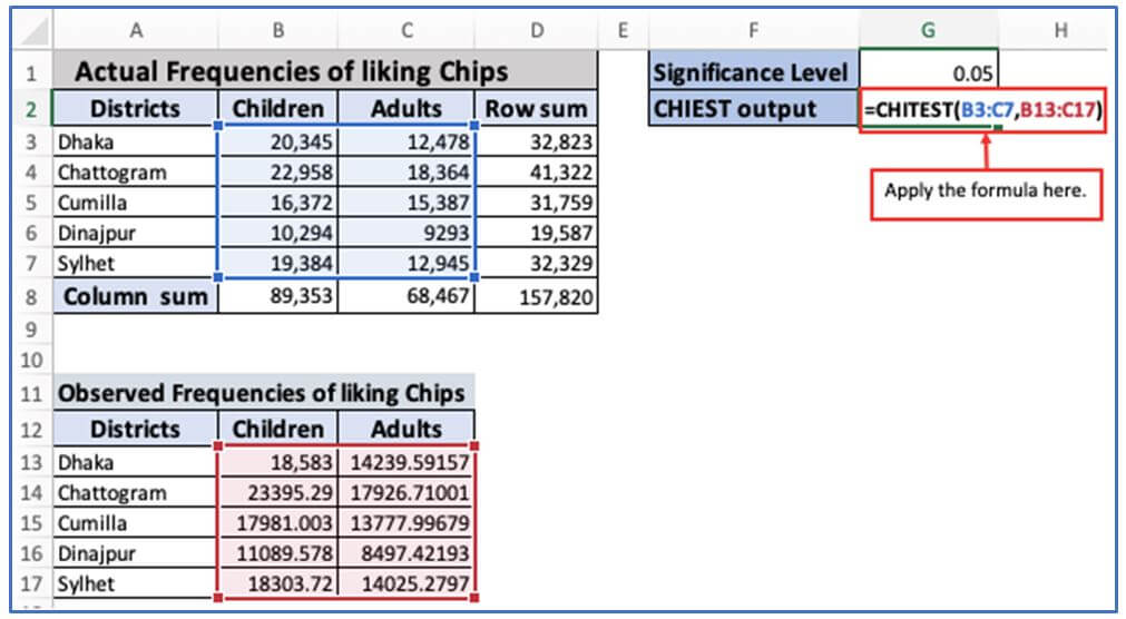
Step 18: Now, enter the CHIEST function formula in cell G2. The formula: =CHITEST(B3:C7,B13:C17)

The formula has been entered here.

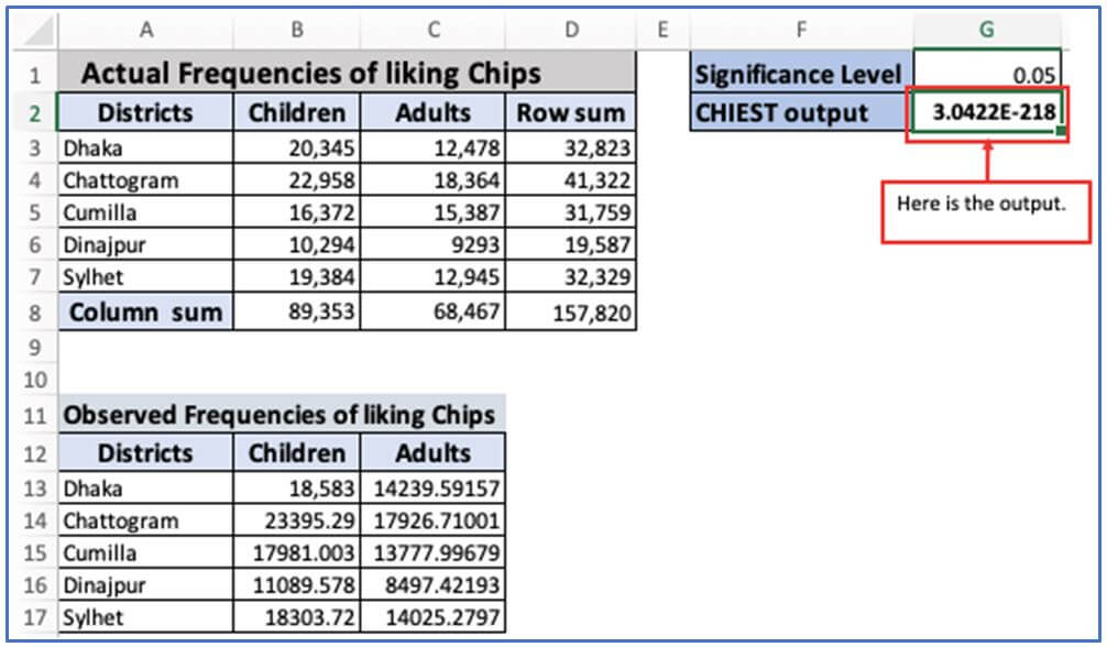
Step 19: This value is very close and is usually displayed as a p-value in the CHIEST test when the observed data is very unlikely under the null hypothesis. There are probably very large test statistics. This means there is a big difference between the observed and expected values. The importance of these outcomes makes it virtually impossible to achieve them by chance (under the null hypothesis). However, they are significant. There is no difference between observed and expected data

Here is the CHIEST function output.

5. How to use CHITEST function in excel? Example-2

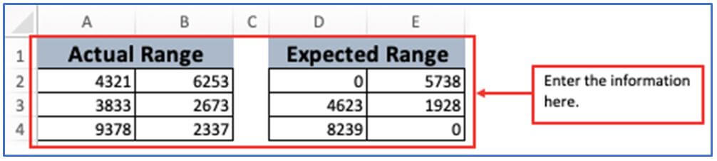
Step 1: Take some information as Actual range and Expected range. First make a data table as shown below.

Entering the data here.

Step 2: Now, add the column in G1 and G2 for getting the result.

The column has been added.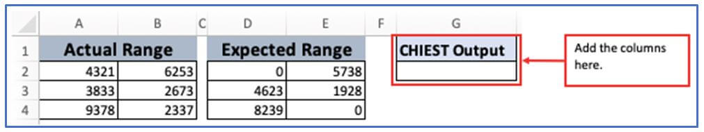

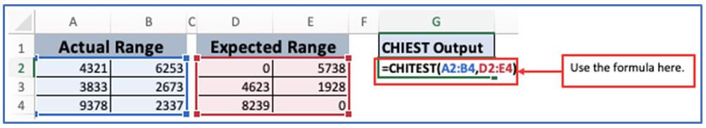
Step 3: Use them CHIEST function formula in cell G2. For this, the formula is: =CHITEST(A2:B4,D2:E4)

Placing the formula here.

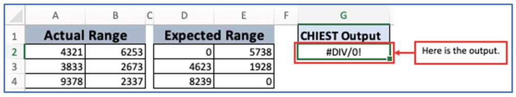
Step 4: After applying the formula press enter and you will get the result. If the field value of the expected area dataset is zero, then CHIEST function will give the output as#DIV/0! Error. You can see in the screenshots that #DIV/0! is shown below whereas computing CHITEST function.

Here is the output of CHIEST function.

6. What are the Common Errors while using CHITEST Function in Excel?

#N/A Error: In most cases, this error indicates that there is a difference between the actual area and the expected area.

#VALUE! Error: The reason for this error could be that it occurs with numerical data in ranges.

Application of CHITEST function in excel

Hypothesis Testing: Evaluate if observed data significantly differs from expected data, supporting statistical hypothesis testing.
Goodness of Fit: Check how well a data set fits a theoretical distribution, helping validate models.
Quality Control: Analyze production defects or errors to determine if variations are due to chance or underlying issues.
Market Research Analysis: Compare survey results with expected outcomes to assess consumer preferences or behaviors.
Genetics and Biology Studies: Test the association between categorical variables, such as gene expression patterns.
Business Forecasting: Validate predictions by comparing expected sales or outcomes with actual results to improve forecasting accuracy.

For ready-to-use Dashboard Templates: