Apply Conditional Formatting to Pivot Tables to revolutionize your data analysis and reporting. By integrating this powerful tool, you can transform complex datasets into clear, intuitive insights. Whether you’re tracking progress, identifying trends, or highlighting key data points, conditional formatting offers a dynamic approach to visualize information effectively. Embrace this feature to make your pivot tables not just more visually appealing, but also significantly more informative and impactful for decision-making. Start today, and see the difference in your data-driven strategies and presentations.
How to Apply formatting to Pivot table cells?
Below are two approaches for ensuring that conditional formatting works even when new data is added.
Option 1: Using the Formatting Icon for Pivot Tables
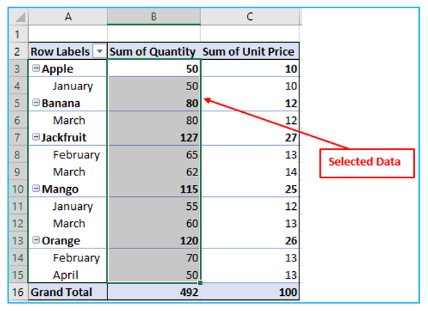
Step 1: Select the cells to which you like to apply conditional formatting.
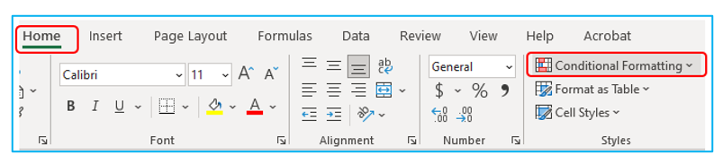
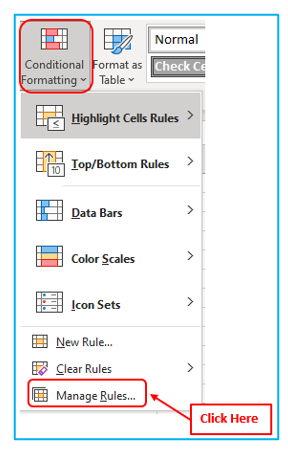
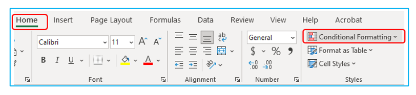
Step 2: Navigate to Home. In the Style area of the ribbon, select the Conditional Formatting.
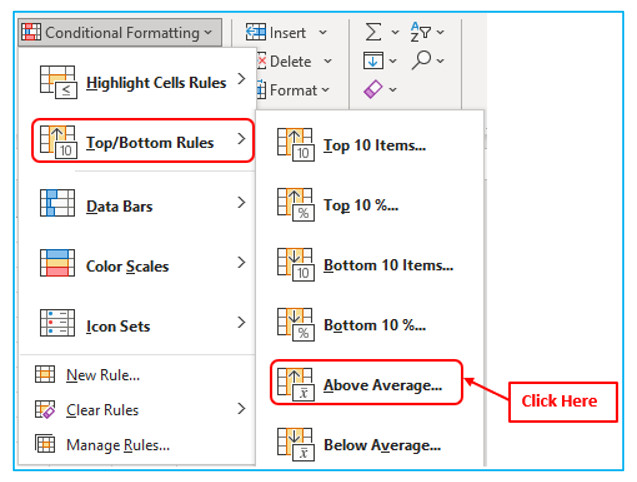
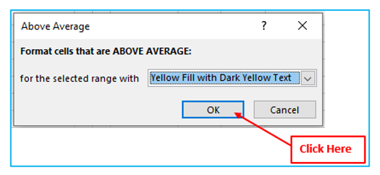
Step 3: Tap on Conditional Formatting, select ‘Top/Bottom Rules’ then click on ‘Above Average’.
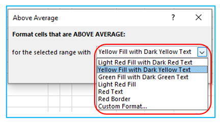
Step 4: Set the format. Then click OK.
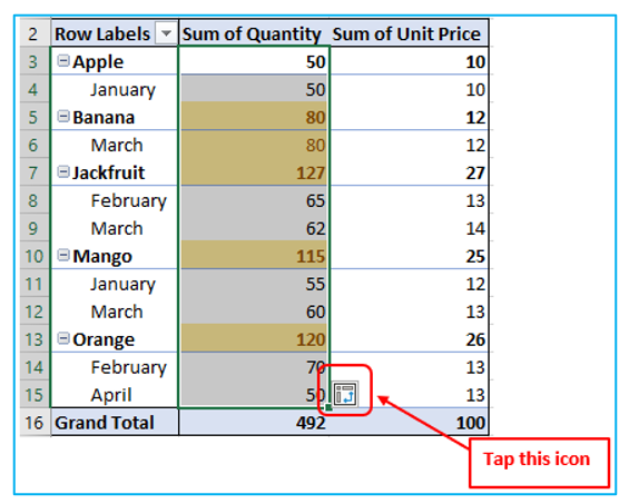
Step 5: At the bottom right of the data collection, it shows the formatting options. Tap that icon.
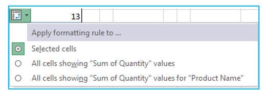
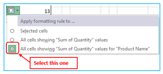
Step 6: It will display three alternatives in a drop-down menu. Choose the third option.
When you add new data and refresh the pivot table, the conditional formatting will instantly cover the new data.
Option 2 – Using Conditional Formatting Rules Manager
Step 1: Select the cell to which you like to apply conditional formatting.
Step 2: Navigate to Home. In the Style area of the ribbon, select the Conditional Formatting.
Step 3: Tap on Conditional Formatting, select ‘Top/Bottom Rules’ then click on ‘Above Average’.
Step 4: Set the format. Then click OK.
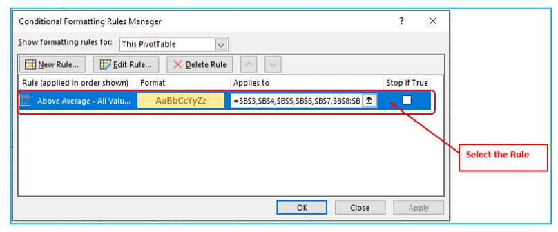
Step 5: Navigate to Home. Select the Conditional Formatting, then go for ‘Manage Rules’.
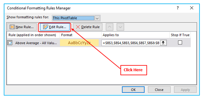
Step 6: Select the rule you wish to update in the Conditional Formatting Rules Manager and click the Edit Rule button.
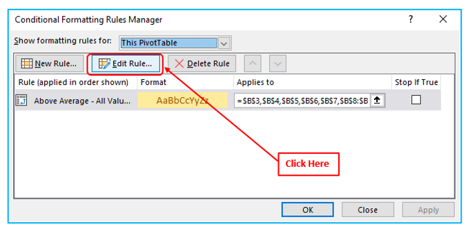
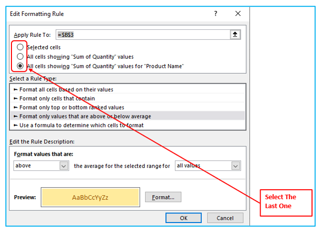
Step 7: You’ll see the exact same three alternatives in the Edit Rule dialogue box. Select the third option.

Step 8: Click OK.
Problems after refreshing the Pivot table
After users apply conditional formatting to a group of cells in the pivot table, the formatting rule is only applied to those cells.
If you later change the pivot table structure or add new records to the source data, it’s possible that it may not contain all of the new data.
How to Fix conditional formatting problem?
After refreshing the pivot table, this step will prevent conditional formatting issues.
Step 1: Select the cell to which you like to apply conditional formatting.
Step 2: Navigate to Home. In the Style area of the ribbon, select the Conditional Formatting.
Step 3: Tap on the Conditional Formatting, then go for ‘Manage Rules’.

Step 4: Select the ‘Rule’ from the Conditional Formatting Rules Manager which you want to change. You can create a new rule or edit an existing rule or delete a rule from here.
Step 5: Click the Edit Rule button
Step 6: You’ll see the three alternatives in the Edit Rule dialogue box. Select the third option.
Step 7: Click OK.
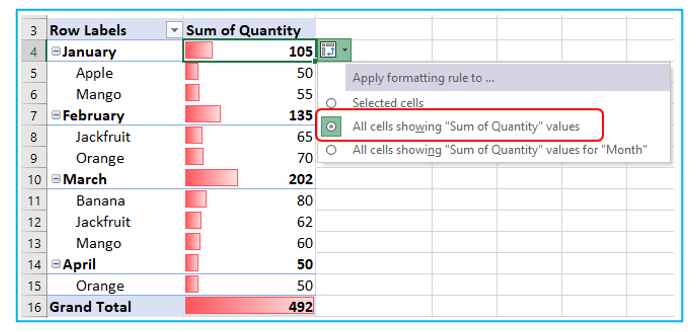
What are the Apply Rule to Options? Understanding the ‘Apply Rule To’.
Understanding the 3 ‘Apply Rule to’ options:
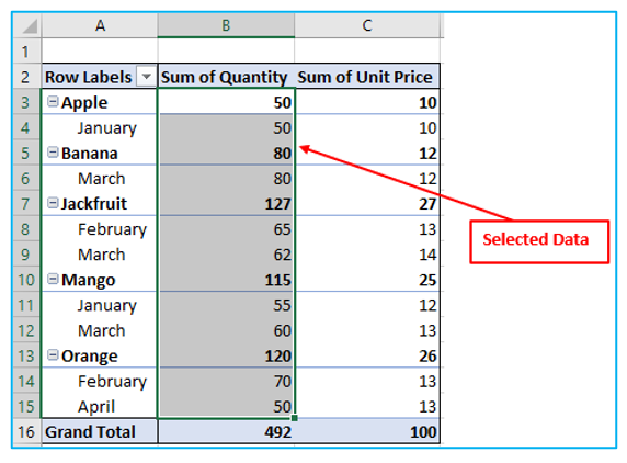
Selected Cells: This option is the default option, in which conditional formatting is applied only to the selected cells.
All Cells Showing “Sum of Quantity” Values: This option takes into account all of the cells that display the Sum of Quantity values (or whichever info that have in pivot table’s values section).
The disadvantage of this option is that it also covers the Grand Total values and applies conditional formatting to them.
All Cells Showing “Sum of Quantity ” Values for “Product Name”: In this scenario, this is the finest option. It applies conditional formatting to all values (excluding Grand Totals). Even though users add additional data in the back end, this option will handle it.
How to Apply Data Bars in Pivot Table? Pivot Table Data Bars.
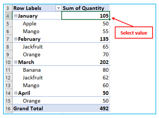
Step 1: Simply select value from the Pivot Table.
Step 2: Navigate to Home. In the Style area of the ribbon, select the Conditional Formatting.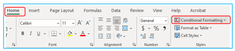
Step 3: Tap on the Conditional Formatting, then go for ‘Data Bars’.
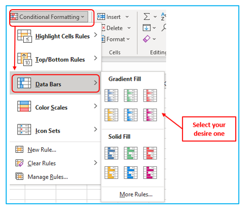
Step 4: To apply the data bar formatting to the full table, go to the Formatting Options Icon and select the second option.
Step 5: Select the third option from the Formatting Options Icon to apply the data bar formatting to the full table while excluding the total column or row
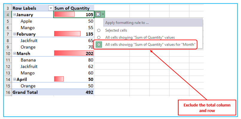
Because the totals do not influence the data bars, users get quite a superior visual representation if they chose the third option.
Application of Apply Conditional Formatting to Pivot Tables
- Highlight Key Data: Use conditional formatting in pivot tables to highlight important information such as top performers, underachievers, or specific numerical thresholds, making critical data stand out at a glance.
- Data Trends Identification: Apply color scales through conditional formatting to visualize data trends and patterns over time within pivot tables, enabling quick identification of increasing or decreasing trends.
- Error and Anomaly Detection: Set up conditional formats to highlight errors, outliers, or anomalies in pivot table data, helping to ensure data accuracy and prompt further investigation.
- Comparative Analysis: Utilize conditional formatting to compare data across different categories or time periods in pivot tables, highlighting differences and similarities with color codes or icons.
- Progress Tracking: Implement conditional formatting to track progress toward goals or benchmarks in pivot tables by color-coding cells based on their proximity to target values.
- Segmentation and Grouping: Use conditional formatting in pivot tables to visually segment and group related data points based on predefined criteria, making complex data sets easier to analyze and understand.
For ready-to-use Dashboard Templates:
