Loan Amortization Schedule in Excel is a powerful tool for managing loans efficiently. By inputting loan details such as principal amount, interest rate, and term, users can generate a comprehensive schedule outlining periodic payments and interest allocations. This feature enables borrowers to visualize their repayment plans, track outstanding balances, and understand the distribution of payments towards principal and interest over time. With its flexibility and customizable options, the Loan Amortization Schedule in Excel empowers users to make informed financial decisions, optimize repayment strategies, and stay on track towards debt repayment goals. Whether for personal budgeting or professional financial analysis, this Excel tool simplifies the complexities of loan management, offering clarity and control throughout the repayment process.
This Tutorial Covers:
- What is the Loan Amortization Schedule
- Preparation of Amortization Schedule in Excel
- Setting up the Amortization Table
- Calculate the Total Payment Amount (PMT Formula)
- Calculate Interest (IPMT Formula)
- Find the Principal (PPMT formula)
- Calculate the Remaining Balance
- Advantages
- Amortization schedule Excel template
1. What is the Loan Amortization Schedule?
The term “loan amortization schedule” refers to a plan for repaying a loan in periodic payments or installments that include both principal and interest payments until the loan term is complete or the whole amount of the loan is repaid.
By using the examples of a vehicle loan and a mortgage, we can clearly comprehend this. In the event of a home loan or auto loan, the lender pays off the balance in a series of installments that are broken down into tiny sums to be paid over a set, significantly longer length of time by generating a loan amortization schedule.
- The interest will be paid initially out of the first few installments that are disbursed. Later on, the installment payment will begin to make up for the principal loan balance.
- In this manner, the lender is able to pay back the loan they borrowed while still covering the interest and principle payments that must be made.
- This is the fundamental notion, and it also holds true when a business organization chooses to take on debt to fund a portion of its operations. Doing so can assist the company operate its operations smoothly with less chance of a financial disaster.
2. Preparation of Amortization Schedule in Excel:
The following functions must be used in order to create an amortization schedule Excel for a loan or mortgage:
PMT function – determines the total amount of a periodic payment using the PMT function. Throughout the whole loan term, this sum does not change.
PPMT function – obtains the portion of each payment that is applied to the loan principle, or the total amount borrowed, using this information. For successive payments, this sum rises.
IPMT function – determines the portion of each payment that is used for interest. Each payment brings down this sum.
How to make Amortization Schedule in Excel is described step by step in the next section.
-
Setting up the Amortization Table:
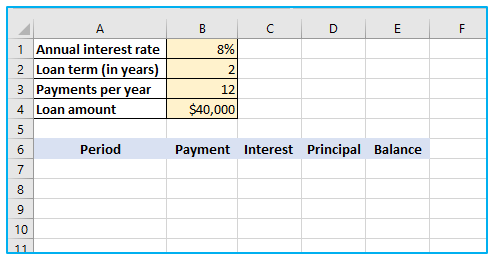
Create the input cells where you will enter the known elements of a loan to begin with:
A1 – annual interest rate
A2 – loan term in years
A3 – number of payments per year
A4 – loan amount
Create an amortization table using the labels Period, Payment, Interest, Principal, and Balance in positions A6 through E6. Enter the total number of payments in the Period field as a series of numbers.
Let’s move on to the most intriguing section, which is loan amortization formulas, given that all the known components are in place.
-
Calculate Total Payment Amount (PMT Formula):
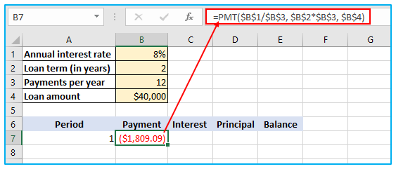
Utilizing the PMT(rate, nper, pv, [fv], [type]) function, the payment amount is determined.
You should be consistent with the values provided for the rate and nper parameters in order to handle various payment frequency (such as weekly, monthly, quarterly, etc.) correctly:
Rate – Divide the annual interest rate ($B$1/$B$3) from the total number of payment periods in a year.
Nper – Multiply the number of years ($B$2*$B$3) by the number of payment periods per year.
Enter the loan amount ($B$4) in the pv parameter.
The default settings for the fv and type arguments are sufficient for us, so they can be ignored. (payments are made at the end of each period, therefore there should be no balance left after the final payment).
The following formula results from combining the aforementioned arguments:
=PMT($B$1/$B$3, $B$2*$B$3, $B$4)
Please note that we have used absolute cell references because the formula should copy exactly to the cells below it.
To determine the first payment, enter the PMT formula in B7.
-
Calculate Interest (IPMT Formula):
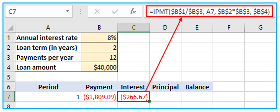
Utilize the IPMT(rate, per, nper, pv, [fv], [type]) function to determine the interest component of each periodic payment:
=IPMT($B$1/$B$3, A7, $B$2*$B$3, $B$4)
With the exception of the per argument, which defines the payment period, all the arguments are the same as in the PMT formula. This parameter is given as a relative cell reference (A7) since the relative position of the row to which the formula is transferred should affect how it changes.
To determine the initial interest, this formula proceeds to C7.
-
Find Principal (PPMT formula):
Use this PPMT formula to determine the principal portion of each periodic payment:
=PPMT($B$1/$B$3, A7, $B$2*$B$3, $B$4)
Similar to the IPMT formula previously explained, the syntax and arguments are precisely the same.
Apply the formula in cell D7 to calculate the first principal part of each periodic payment.
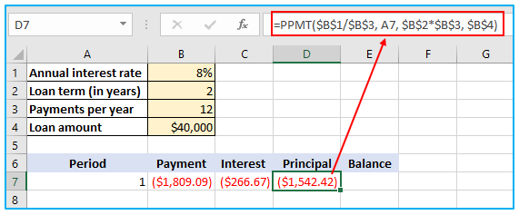
Tip: At this stage, add the figures in the Principal and Interest columns to see if your calculations are accurate. In the same row, the sum must match the value in the Payment column.
-
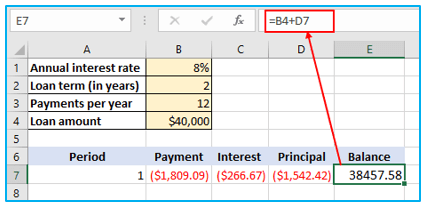
Calculate the Remaining Balance:
We’ll employ two distinct formulae to determine the balance that remains at the end of each session.
Add the loan amount (B4) and the initial period’s principle (D7) together to determine the balance in E7 after the first payment:
=B4+D7
Principal is deducted from the loan amount because it is a negative number while the loan amount is positive.
Now, let’s calculate the rest: payment, interest, principal, and balance.
Drag down one row while selecting the range A7:E7 (initial payment). Adjust the formula for the balance and the updated formula is as follows:
=E7+D8
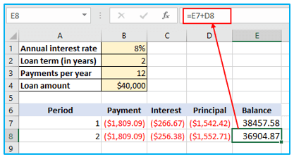
To extend the formula for the second payment in range A8:E8 until the balance reaches zero using auto fill handler.
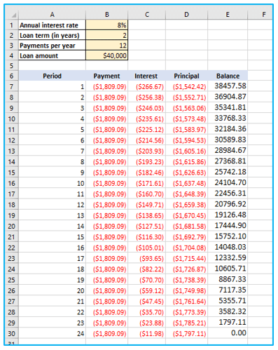
As each payment is made towards the loan, the allocation of the payment amount between the principal and interest changes. Over the course of 24 months, the principal portion of the payment will increase while the interest portion will decrease.
This phenomenon occurs because in the early stages of the loan, a larger portion of the payment goes towards the interest, while only a small part is allocated towards the principal. As more payments are made, the outstanding principal balance reduces, resulting in a smaller interest component and a larger principal component.
Therefore, by the end of the loan term, the majority of the payment amount will be applied towards the principal, reducing the overall amount owed on the loan.
3. Advantages:
A company organization can profit greatly from the practice of amortization in many different ways. The strategy of dividing up a mortgage or debt that the company has can assist the company repay it while experiencing less stress. The borrower’s ability to repay the loan without interfering with other business operations is further aided by the loan amortization plan. There is no need to make a large upfront investment because the repayment is provided in terms.
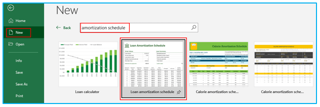
4. Amortization schedule Excel template:
Use Excel’s built-in templates to quickly create a top-notch loan amortization schedule. Simply select the template you want by choosing File > New and typing “amortization schedule” into the search box.
Then you may reuse the freshly produced workbook whenever you want by saving it as an Excel template.
This is how you make an Excel amortization schedule for a loan or mortgage.
Application of Loan Amortization Schedule in Excel
- Payment Schedule: A loan amortization schedule in Excel helps to organize and visualize the repayment schedule of a loan, detailing each payment’s amount, date, and allocation between principal and interest.
- Principal and Interest Breakdown: It calculates the breakdown of each payment into principal and interest components, allowing users to understand how much of each payment goes towards reducing the loan balance and paying interest.
- Total Interest Paid: It calculates the total amount of interest paid over the life of the loan, providing insights into the overall cost of borrowing.
- Remaining Balance: It tracks the remaining balance of the loan after each payment, helping borrowers stay informed about how much they still owe and when the loan will be fully repaid.
- Comparison of Scenarios: Users can compare different loan scenarios by adjusting variables such as interest rate, loan term, and payment frequency to see how changes impact the repayment schedule.
- Analysis of Extra Payments: The schedule accommodates additional payments, allowing users to analyze the effects of making extra payments towards principal on the overall loan term and interest savings.
For ready-to-use Dashboard Templates:
