Transpose in Excel offers a seamless solution for rearranging data, transforming columns into rows and vice versa with ease. Whether you’re reorganizing datasets, converting data for analysis, or preparing reports, Transpose in Excel simplifies the process, saving you time and effort. Say goodbye to manual data rearrangement and hello to efficiency with this powerful feature. From streamlining data entry to optimizing data visualization, Transpose in Excel enhances your workflow, empowering you to work smarter, not harder. Take control of your data presentation and analysis by leveraging the versatility of Transpose in Excel. With just a few clicks, you can reshape your data to fit your needs, unlocking new possibilities for data manipulation and interpretation. Embrace the convenience and flexibility of Transpose in Excel and elevate your spreadsheet skills to new heights of productivity and efficiency.
This Content Covers:
- What is Transpose in Excel?
- How Do We Transpose in an Excel Worksheet?
- Transpose Data using Paste Special Dialogue Box
- Power Query to Transpose Data in Excel
- Transpose Data using a Keyboard Shortcut
- Transpose Data using the Transpose Option
- Transpose Data using Transpose Function
- Use of TRANSPOSE Function with IF Statement
- TRANSPOSE Function to add Prefix
- How to Delete TRANSPOSE Function from an Excel Worksheet?
1. What is Transpose in Excel?
Transposing basically refers to the process of making two or more objects take the place of one another. This is used to convert rows into columns and columns into rows while working with data in Excel. Excel’s TRANSPOSE feature makes it easier to swap (rotate) the values between rows and columns and vice versa. Its role is to arrange the data in the preferred format.
2. How Do We Transpose in an Excel Worksheet?
Now we will see what the best ways are that we can use to transpose data in Excel.
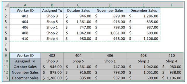
2.1 Transpose Data using Paste Special Dialogue Box
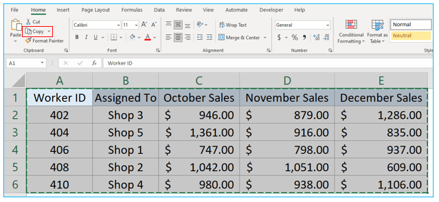
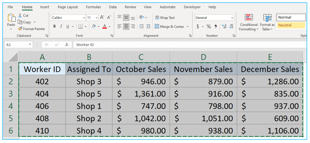
Step 1: First select the data that you want to transpose and then click on the Copy option from Home tab or press CTRL+C shortcut to copy the data.
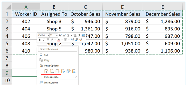
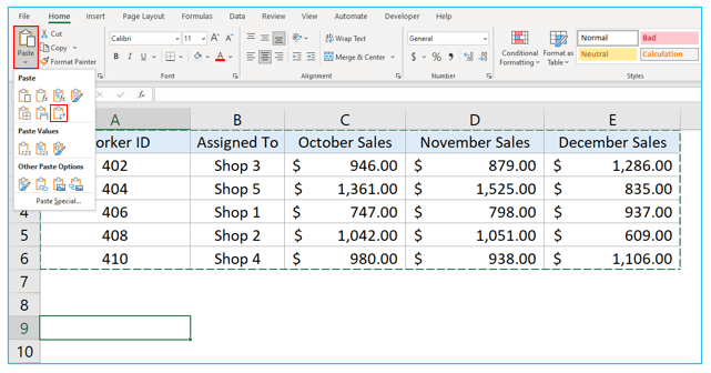
Step 2: Right click on a cell where you want to paste the transposed data and select Paste Special option. Or after selecting the cell, press CTRL+ALT+V shortcut keys to open Paste Special dialogue box.
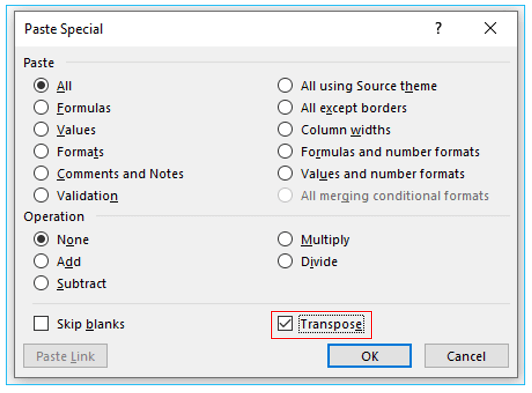
Step 3: Check the Transpose box and press OK.
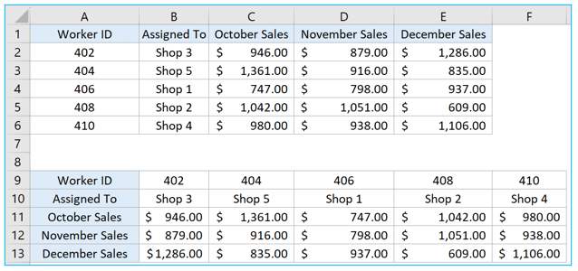
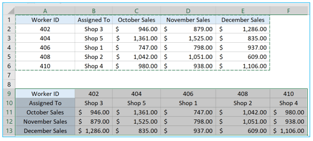
Step 4: The transposed data is now pasted in that selected cell.
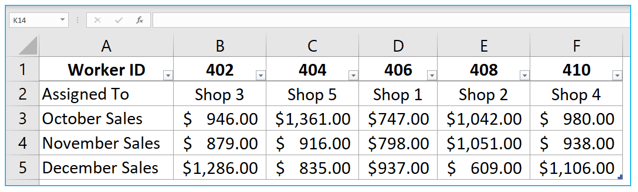
2.2 Power Query to Transpose Data in Excel
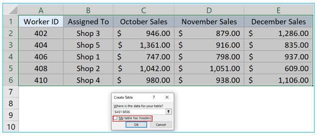
Step 1: To use the data in power query, first you need to make sure the data is in table form. If it is a tabular data that you are working with then convert it into a data table by selecting the data and pressing CTRL+T shortcut keys to open Create Table dialogue box. Make sure My table has headers box is unchecked before you press OK.
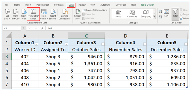
Step 2: Select any cell from the table then go to Data tab and select From Table/Range. This will open the Power Query Editor.
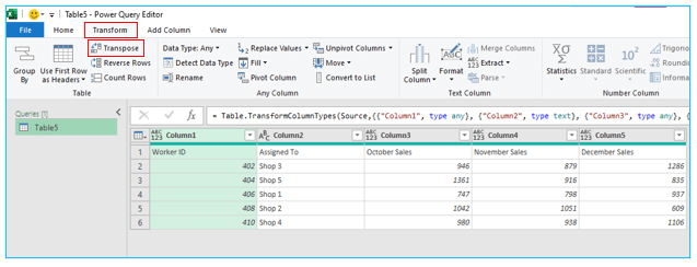
Step 3: Click on Transform tab inside Power Query Editor and press the Transpose option.
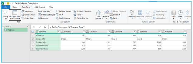
Step 4: Now click on Use First Row as Headers option to use the first row as header. The data is now transposed successfully.
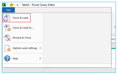
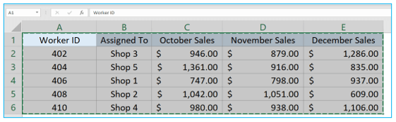
Step 5: Click on File and then press Close & Load option. This will display the transposed data onto another sheet.
Step 6: Now open the other sheet to see the result.
2.3 Transpose Data using a Keyboard Shortcut
Step 1: First select the whole range and copy it using CTRL+C.
Step 2: Then select a cell where you want to paste the data and press ALT+H+V+T shortcut keys one after another.
Step 3: This will transpose the data and paste it in that cell.
2.4 Transpose Data using the Transpose Option
Step 1: Select the entire range and copy using CTRL+C.
Step 2: Select a cell where you want to paste the data, then go to Home tab and click on Paste option. Select Transpose from the drop-down list.
Step 3: When you click on the Transpose option, the data will be transposed in this cell.
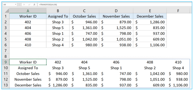
2.5 Transpose Data using Transpose Function
Using TRNASPOSE function in Excel 365 is very easy as it can work with dynamic array formulas very easily. But working in other versions of Excel and using TRANSPOSE function is a bit tricky. Let’s see how the TRANSPOSE function works in the simplest of ways.
Step 1: Select a cell where you want the data to be transposed and pasted. Then insert this formula in that cell.
=TRANSPOSE(range)
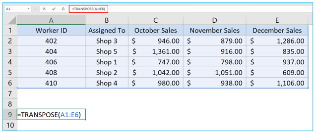
Step 2: Press Enter key and the data will be transposed here. The tricky part is, if you are using Excel 365 then only pressing Enter key will do the trick. But if you are using any other version of Excel and the array is a dynamic array then pressing Enter key won’t give you the correct result. Instead of Enter, you must press CTRL+SHIFT+ENTER keys in other versions of Excel.
2.6 Use of TRANSPOSE Function with IF Statement
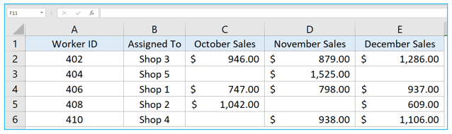
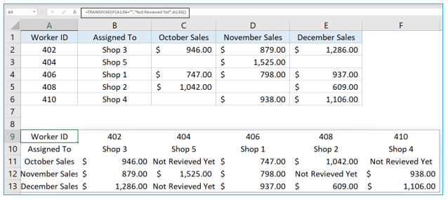
Suppose we haven’t received the sales data for some of the cells in this table. Now if we use TRANSPOSE function in this table, the transposed data will also show blank cells for those cells. If we want to use any text as a string such as “Not Received Yet” or a Zero instead of blank cells, we can use the IF statement with TRANSPOSE function to do that.
Step 1: Select a cell where you want the data to be transposed and pasted. Then insert this formula in that cell. Press Enter key to see the result. Press CTRL+SHIFT+ENTER keys if you are using other versions of Excel.
=TRANSPOSE(IF(A1:E6=””,”Not Revieved Yet”,A1:E6))
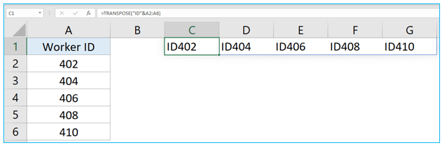
2.7 TRANSPOSE Function to add Prefix
Step 1: Suppose we want to transpose only the data of column A and add a prefix to this data. We can do this very easily using the TRANSPOSE function. Select a cell and insert this formula in the cell.
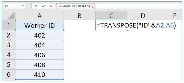
Step 2: Press Enter key to see the result.
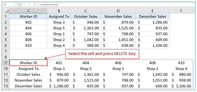
3. How to Delete TRANSPOSE Function from an Excel Worksheet?
Step 1: To remove the TRANSPOSE function all you need to do is select the first cell of the table where you have inserted the formula and then press Delete key from your keyboard.
Application of Transpose in Excel
- Data Reorganization: Easily restructure data by converting rows into columns or vice versa using Transpose in Excel, facilitating better organization and analysis.
- Reshaping Data: Transform datasets to meet specific formatting requirements or to integrate with other software applications efficiently.
- Data Consolidation: Combine data from multiple sources or worksheets by transposing it into a single, unified format for easier comparison and analysis.
- Chart Creation: Prepare data for charting or graphing purposes by transposing it to align with the desired axis or series format, enhancing visualization clarity.
- Reporting: Convert data for reporting purposes, such as summarizing monthly sales figures or quarterly financial data, into a more concise and readable format.
- Database Import/Export: Adjust data layouts to match database schema requirements when importing or exporting data between Excel and other databases, ensuring seamless data integration.
For ready-to-use Dashboard Templates:
