Lock, Hide Cells, and Protect Worksheet in Excel to ensure your data’s security and integrity. This crucial feature allows you to safeguard sensitive information, maintain spreadsheet functionality, and control user interactions. By implementing these protective measures, you can prevent unauthorized access and modifications, ensuring that your data remains accurate and confidential. Embrace the full potential of Excel’s security features to create a more secure, reliable, and user-friendly data management environment. Start protecting your worksheets today to keep your data safe and sound for tomorrow’s needs.
How to lock all cells?
All cells are locked by default. However, until you protect the worksheet, cell locking is ineffective.
Procedure of locking all cells are as follows:
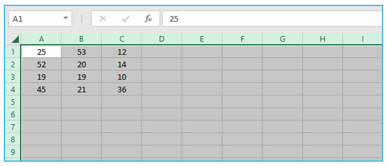
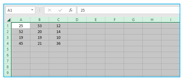
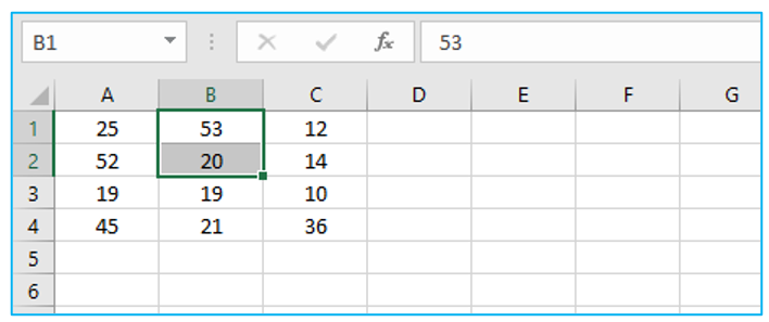
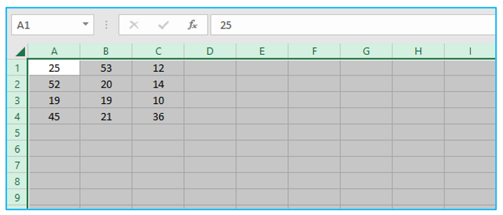
Step 1: Select all cells, outlined in Blue below.
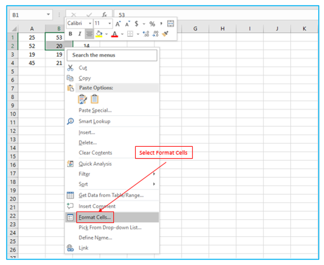
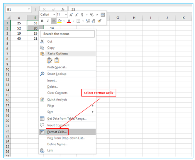
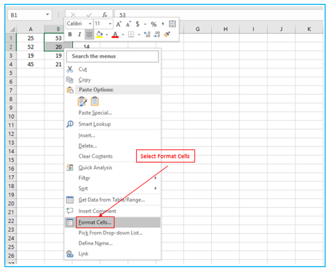
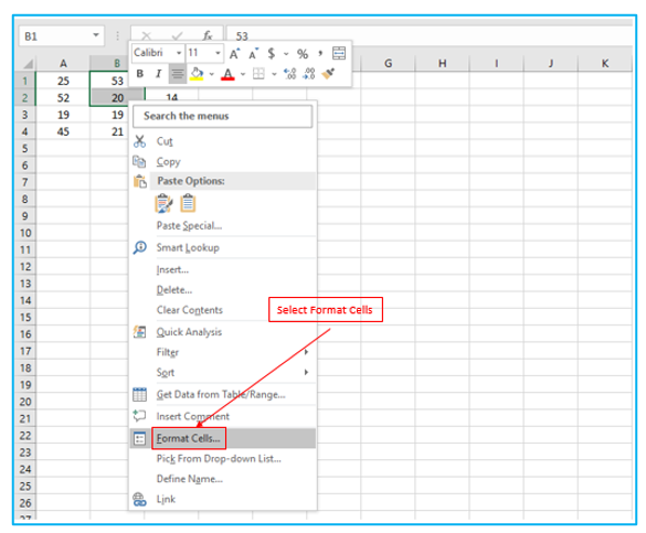
Step 2: Format Cells can be selected by right-clicking or by pressing CTRL + 1, outlined in Red below.
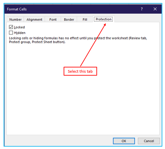
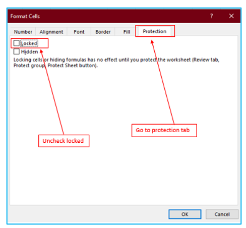
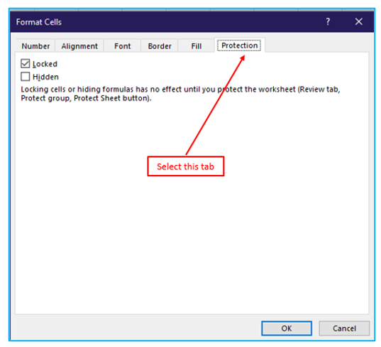
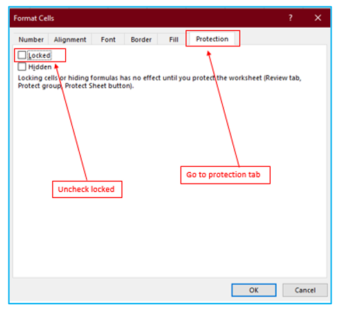
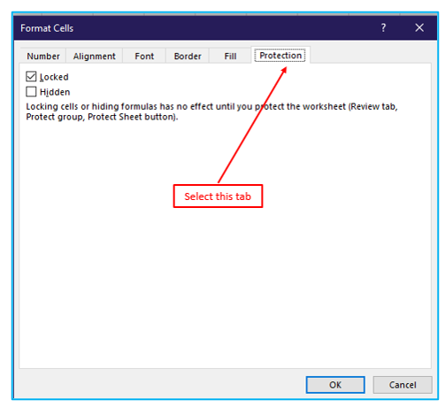
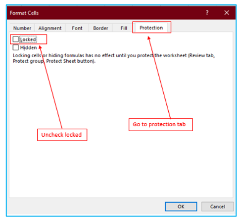
Step 3: You can check to see if all cells are locked by default on the Protection tab, outlined in Red below.
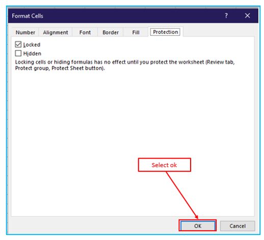
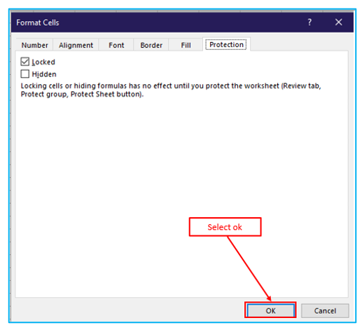
Step 4: Click ok, outlined in Red below.
How to protect worksheet in Excel?
Users of Microsoft Excel may quickly track, store, and manage data using this program. By securing worksheets, lock cells prevent unwanted data alterations. To assist prevent it from being altered, you might want to safeguard a worksheet when you share an Excel file with other users.
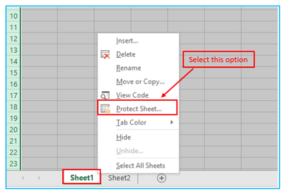
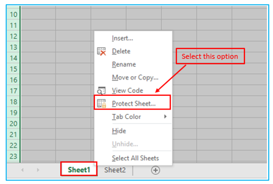
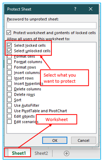
Procedure of protecting worksheet as follows:Step 1: Right click a worksheet tab (For example, Sheet1) and click “Protect Sheet”, outlined in Red below.
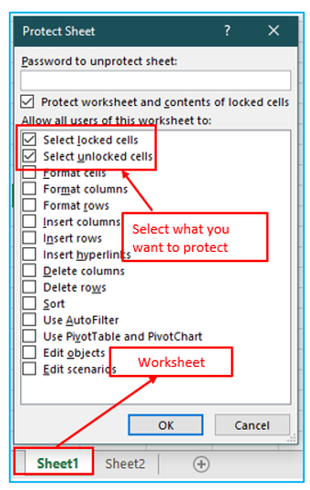
Step 2: Select what you want to protect, type password and click ok, outlined in Red below.
How to lock specific cells?
In Excel, unlock all cells before locking any particular ones. Lock particular cells next. Protect the sheet lastly.
Procedure of locking all cells are as follows:
Step 1: Select all cells, outlined in Blue below.
Step 2: Format Cells can be selected by right-clicking or by pressing CTRL + 1, outlined in Red below.

Step 3: Uncheck the Locked check box on the Protection tab, then select ok, outlined in Red below.
Step 4: For example, select cell B1 and cell B2, outlined in Green below.
Step 5: Format Cells can be selected by right-clicking or by pressing CTRL + 1, outlined in Red below.
Step 6: You can check to see if all cells are locked by default on the Protection tab, outlined in Red below.
Step 7: Click ok, outlined in Red below.
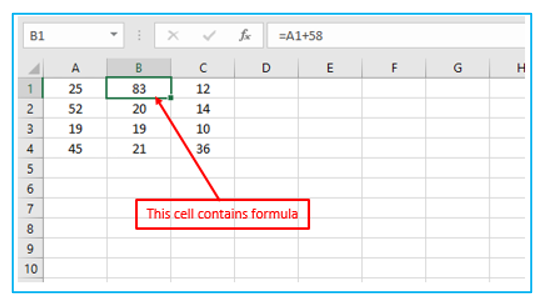
How to lock formula cells?
All cells must first be unlocked before locking any cells that have formulas. Lock each formula cell after that. Protect the sheet lastly.
Procedure of locking all formula cells are as follows:
Step 1: Select all cells.

Step 2: Format Cells can be selected by right-clicking or by pressing CTRL + 1.

Step 3: Uncheck the Locked check box on the Protection tab, then select ok.
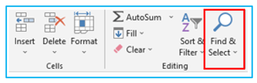
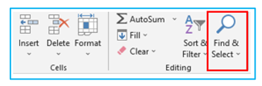
Step 4: On the Home tab, click Find & Select.
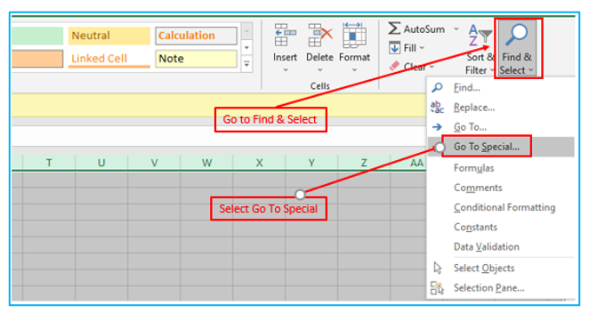
Step 5: Click “Go To Special”, outlined in Red below.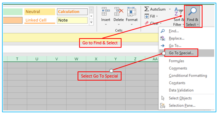
Step 6: Select Formulas and click ok.
Step 6: Select Formulas and click ok.
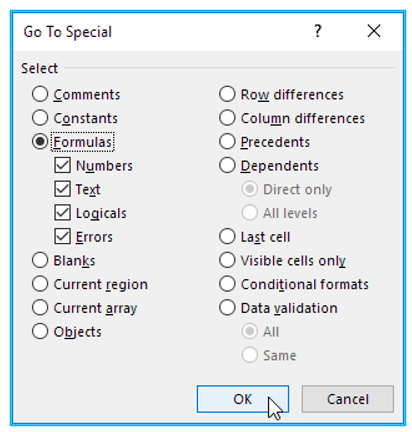
Microsoft Excel selects all cells that contains formula automatically, outlined in Red below.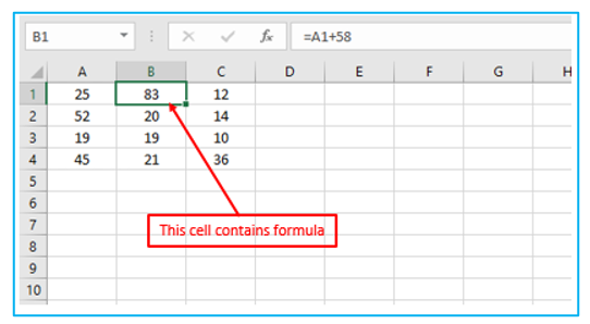
Step 7: Format Cells can be selected by right-clicking or by pressing CTRL + 1, outlined in Red below.
Step 8: Check the “Locked” box on the Protection tab and then click ok.
How to lock and hide formulas?
Using specified data in a particular order, a function is a pre-set formula that conducts calculations. Common functions that can be used to rapidly determine the sum, average, count, maximum value, and minimum value for a range of cells are included in all spreadsheet systems.
Procedure of locking and hiding formulas are as follows:
Step 1: Select all cells.
Step 2: Format Cells can be selected by right-clicking or by pressing CTRL + 1.

Step 3: Uncheck the Locked check box on the Protection tab, then select ok, outlined in Red below.
Step 4: On the Home tab, click Find & Select, outlined in Red below.
Step 5: Click “Go To Special”, outlined in Red below.
Step 6: Select Formulas and click ok.
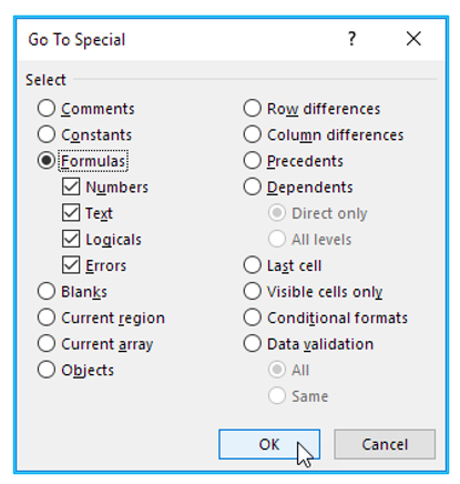
Microsoft Excel selects all cells that contains formula automatically, outlined in Red below.
Step 7: Format Cells can be selected by right-clicking or by pressing CTRL + 1.
Step 8: Check the “Locked” and “Hidden” box on the Protection tab and then click ok, outlined in Red below.
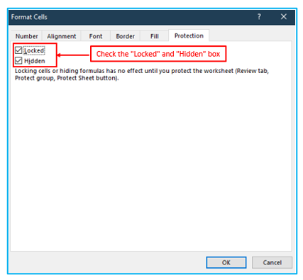
Even if cells are locked and hidden, the worksheet must first be protected before the changes take effect.
So, worksheet should be protected.
Procedure of protecting worksheet as follows:
Step 1: Right click a worksheet tab (For example, Sheet 1) and click “Protect Sheet”, outlined in Red below.
Step 2: Select what you want to protect, type password and click ok, outlined in Red below.
Application of Lock, Hide Cells and Protect Worksheet in Excel
- Data Security: Lock cells to prevent unauthorized users from editing sensitive information, ensuring data integrity and security within your Excel worksheets.
- Confidentiality Maintenance: Hide cells containing confidential or sensitive data, such as personal details or financial information, to restrict visibility only to authorized users.
- Formula Protection: Protect formulas in your worksheet to prevent accidental deletion or alteration, maintaining the accuracy and reliability of your data calculations.
- Structural Consistency: Protect the entire worksheet to maintain its structure, preventing users from adding, deleting, or resizing rows and columns, which could disrupt the layout or functionality.
- Input Control: Lock all cells except for designated input areas to guide users on where they can enter data, reducing the risk of accidental changes to critical data.
- Version Control: Protect the worksheet to ensure that changes are made only by individuals with the correct permissions, aiding in version control and the prevention of unauthorized alterations.
You may be interested:
