Compound interest is calculated when a deposit, loan, or interest is added to the principal amount. It is the result of reinvesting interest such that it is received in the principal amount plus accrued interest over the subsequent period. This can be easily calculated using an Excel sheet with the compound interest formula for Excel,which is FV=PV(1+r)n.
In the compound interest formula for Excel, PV stands for current value, r is for the interest rate per period, FV is for future value, and n is for the number of compounding periods. Let us see how we can use this formula and calculate the compound interest in Excel.
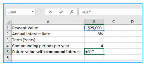
Using Mathematical Compound Interest Excel Formula
- Step 1: Multiply the principal amount by the interest rate.
- Step 2: Now, divide the yearly interest rate by the compounding periods per year.
- Step 3: Then, reference a cell containing the number of years to multiply the compounding periods per year by that number.
- Step 4: The result will be displayed after pressing Enter.
How to Use a Compound Interest Calculation Table in Excel?
- Step 1: The name of the cell containing the value of the annual interest rate should be changed to ‘Rate’ by using the Name Box.
- Step 2: Then multiply the principal amount by the yearly interest rate divided by the compounding periods per year. This will give you the investment’s value at the conclusion of the first quarter.
- Step 3: The result will be shown after applying the formula.
- Step 4: Then, fill all the cells and pull the ‘Fill Handle’ further.
Using the FVSCHEDULE Excel Formula
- Step 1: Enter the annual interest rate reference for ‘primary’ and interest rate for ‘schedule, respectively, since it is the result of dividing the annual interest rate by the compounding periods per year.
- Step 2: The result will be shown after applying the FVSCHEDULE formula.
Calculating Compound Interest Using FV Excel Formula
In this method, the Annual interest rate divided by compounding periods per year will be used to determine the rate. Let us see how.
- Step 1: First, the value of ‘nper’ should be defined as Term*Compounding periods per year.
- Step 2: For ‘pmt”, enter 0 as no extra principle value increments will be made between the investing periods.
- Step 4: Once the value for ‘pmt’ has been eliminated, you will get the initial investment or the present value. This will be used with a PV reference that has a negative sign.
- Step 5: After pressing ‘Enter,’ you will get the result as the future value along with the compound interest.
Keep This in Mind When Using Compound Interest Formula for Excel
Ensure you enter the interest rate in either decimal or percentage form.
You need to specify the ‘PV’ and ‘PMT’ inputs in the FV function in the negative form.
The FV function will return the #VALUE. So, any non-numeric value provided as an argument will give an error.
Either PV or PMT inputs should be mentioned in the FV function.
Conclusion
These are the ways you calculate compound interest in Excel by using the compound interest formula in Excel. Ensure that you follow all the steps thoroughly to avoid any errors.