

A chart isn’t advanced just because it looks polished. Advanced Excel charts and graphs make data easier to interpret, compare multiple data sets, or respond dynamically to a viewer’s choices. Percentage-change annotations, scrollable views, and zoom controls are practical examples: each can reveal a pattern or detail that a basic chart may leave harder to see.
It’s frustrating when a chart contains the right data but still makes comparisons difficult. The solution isn’t complexity for its own sake; it’s choosing a feature that answers a clear question. In this article, you’ll learn what makes an Excel chart advanced and see how percentage-change labels clarify movement over time. You’ll also explore how scrolling and zoom controls can make dense or multi-chart views easier to navigate. Use these ideas to create visuals that are engaging and useful to the people who rely on them.
Key Takeaways
- Choose a chart based on the comparison or pattern you want readers to understand, not just how the data is arranged.
- Use percentage-change annotations and contrasting colors to make rises and falls easier to spot.
- Add scrolling or zoom controls when readers need to explore detailed data or focus on one chart at a time.
- A chart becomes advanced when its design helps people compare, explore, or interpret data more effectively.
What is an advanced Excel Chart?
An advanced chart does more than display values: it helps readers compare data sets, track change, or explore details. Choose a format by asking what decision the visual should support. Use a line chart for change over time, columns to compare periods, and a doughnut chart to show progress toward a goal. For a dashboard comparing actual results with several targets, use horizontal or vertical bars and add attainment percentages.
Situation: a stacked bar chart shows each department’s contribution to total sales, but the series are difficult to compare because their baselines differ. Action: add dynamic data labels that let viewers switch which series values are displayed. Result: readers can focus on the department they need to compare instead of interpreting every label at once. A comparative distribution chart can also show one category against others across multiple series.
A 3-D effect adds depth to a data series, but it can make values harder to judge because perspective changes apparent size. Situation: a column chart compares product totals. Action: test the 3-D view against a flat version and keep it only if the added depth improves the message. Result: viewers can compare values without mistaking visual perspective for a data difference.
Microsoft 365, Excel 2024, and older releases can differ in available chart types and interface. Excel 2016 added Histogram as a default chart type, while charting techniques demonstrated for Excel 2013, 2016, 2019, and 365 apply to those versions.
To make a dynamic chart, format the source data as an Excel table, then build the chart from its columns. Adding rows to the table expands the chart data. Named ranges or formulas can also define changing chart ranges.
For a combo chart, select the data, choose Insert and Combo Chart, then assign a chart type to each series. Put a series with a different scale, such as revenue and percentage growth, on the secondary axis.
To show a trendline, select a data series, open Chart Elements, and add a trendline. Use its formatting options to set a forecast period or display the equation on the chart.
For custom error bars, select the series, open Chart Elements, choose Error Bars, then select More Options and Custom to specify positive and negative ranges. Use a box-and-whisker chart to show distribution. Excel’s built-in chart options and formatting vary by version.
Avoid 3-D effects that distort comparisons, crowded labels, and mismatched scales. Before sharing a dashboard, check that each chart’s title, axis, values, and legend support the same clear takeaway.
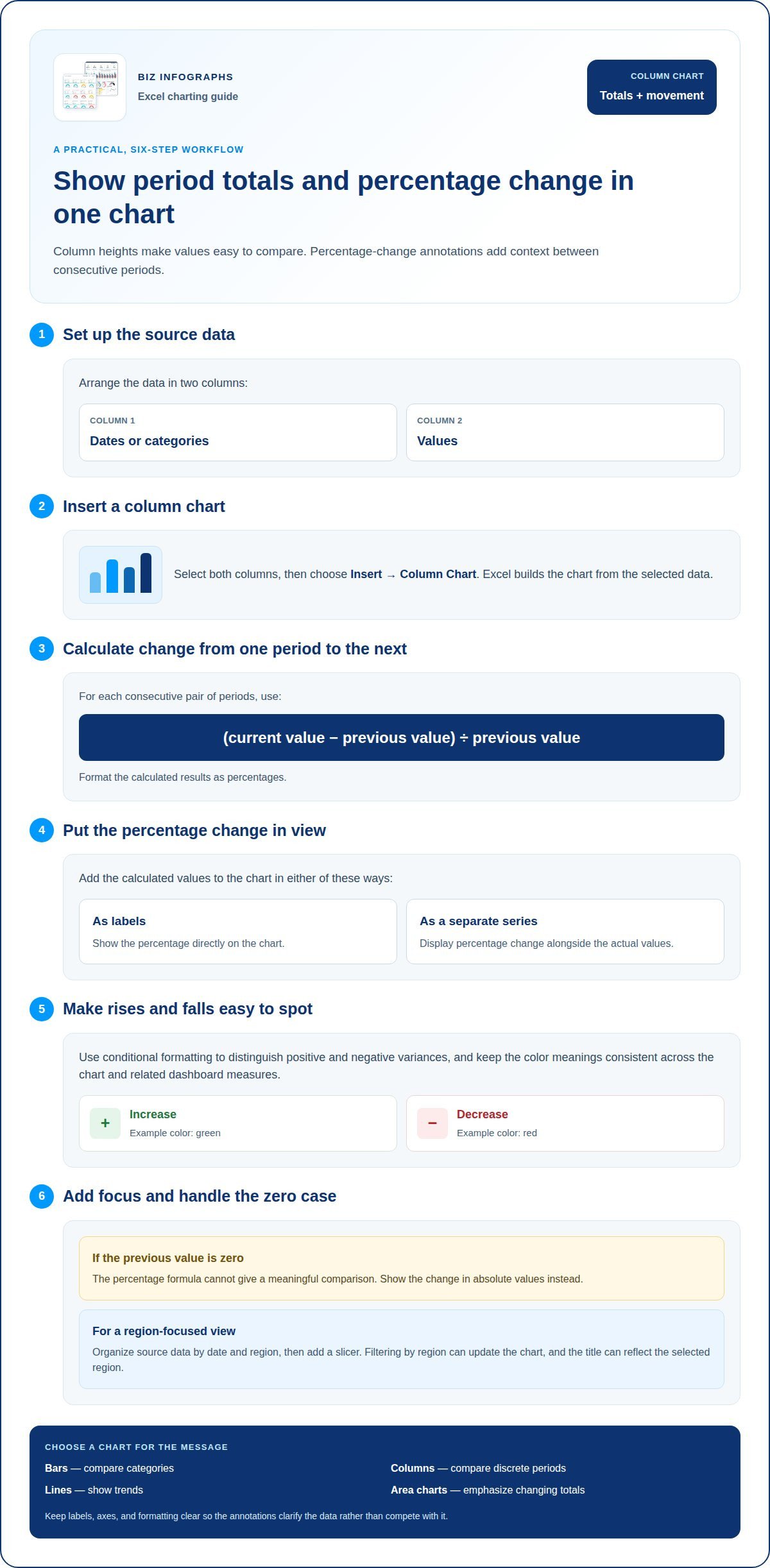
Column charts with percentage-change annotations
A column chart compares values across periods or categories; percentage-change annotations add context between consecutive periods. Begin with dates or categories in one column and values in another. Select both columns, then choose Insert and a column chart. Excel builds the chart from the selected data, making the underlying values easy to compare.
Situation: a monthly sales chart shows each period’s total, but readers also need to spot month-to-month changes. Action: calculate each change as (current value − previous value) ÷ previous value, then format the results as percentages. Add the calculated values as labels or a separate chart series. Result: the chart shows both actual totals and relative movement between periods.
Use conditional formatting to distinguish positive and negative variances with different colors. For example, show a sales increase in green and a decrease in red, with the annotation displaying the calculated percentage. Keep color meanings consistent across the chart and any dashboard using the same measures. If the previous value is zero, the percentage formula cannot give a meaningful comparison, so show the change in absolute values instead.
To keep the chart responsive, organize source data by date and region, then add a slicer. Filtering by region can update the chart, and the title can reflect the selected region. Readers can explore a focused comparison without rebuilding the visual.
Match chart type to the message: bars compare categories, columns compare discrete periods, lines show trends, and area charts emphasize changing totals. Pie and doughnut charts show parts of a whole, but use them when the slices support a clear comparison. For a percentage-change story, columns make period-to-period movement easy to scan. Refine labels, axes, and formatting so annotations clarify the data rather than compete with it. Explore Excel chart examples for more visual approaches.
Interactive charts with scroll and zoom controls
Interactive charts let viewers explore a focused slice of data instead of scanning every value at once. Situation: a dashboard contains several small charts, and a reader needs to inspect one. Action: use a chart macro to add a button that enlarges one chart at a time. Result: the selected visual is easier to read without permanently changing the dashboard layout.
To build an interactive dashboard with slicers and PivotCharts, summarize a structured data range in a PivotTable, then insert a PivotChart. Add a slicer from PivotTable Analyze, choose a field such as region, and connect it to relevant PivotTables through report connections. Selecting an item in the slicer filters the connected charts together.
A scroll bar can control the grouping in a dynamic histogram. Situation: a distribution chart needs to show different numbers of groups. Action: insert a scroll bar form control, link it to a worksheet cell, and use that cell in formulas defining the histogram bins. Result: moving the control changes the grouping. Selecting a group can also drive a detailed report of its entries.
For changes at irregular intervals, use a step chart rather than implying continuous movement. Situation: a price changes only on particular dates. Action: prepare repeated date-and-value points that hold each level steady until the next change, then plot them in an XY scatter chart with straight lines. Result: the steps show exactly when each change occurred.
A waterfall chart shows how increases and decreases bridge a starting value to an ending value. Select the category and amount columns, then choose Insert and Waterfall; mark starting and ending totals as totals. For interactive exploration, connect its source to filtered data so selected categories update the bridge. To create a funnel, select stage names and values, then insert a Funnel chart. To create a histogram, select numeric values and insert Statistic Chart and Histogram; Excel 2016 added Histogram as a default chart type. Conditional formatting can reinforce key changes, while clear labels keep each interactive view readable.
What qualifies as an advanced Excel chart
An advanced chart earns its complexity by helping readers interpret data more clearly. A polished color palette alone doesn’t qualify. Look for a useful capability: comparing multiple data sets, revealing changes, or letting viewers explore a focused view. For example, an annual trend chart can compare two time increments with past averages, giving readers more context than a single-period snapshot.
Situation: a team tracks progress toward a target, but a static graphic hides whether performance is improving. Action: use a conditional doughnut chart that changes color as the displayed percentage increases. Result: viewers can recognize progress and status at a glance. The color shift should support the value, not replace a clear label explaining what the chart measures.
Comparison can also make a chart advanced. Imagine a report with actual results and several targets. Display the values horizontally or vertically, then add an attainment percentage showing how actual performance compares with each goal. Conditional formatting can distinguish favorable and unfavorable results using consistent colors. This adds analytical meaning, not just decoration, by linking each result to its benchmark.
Situation: a report compares categories across several data series, but readers need to see one category’s distribution against the others. Action: use a comparative distribution chart to show the segment across those series. Result: the visual enables comparisons that might otherwise require quartile plots or multiple histograms.
Use this test before adding a feature: does it answer a specific reader question? If dynamic labels improve series comparisons, or a chart makes actual-versus-target performance clearer, the added design has a purpose. If a 3-D treatment only changes appearance, it adds complexity without improving interpretation. Advanced Excel charts and graphs combine relevant data, clear visual encoding, and useful interaction. Choose colors consistently, label measures plainly, and keep the takeaway easy to identify.
Build your next report around that principle with ready-to-use Excel chart designs that help turn values into clearer visual comparisons.
Biz Infographs: PowerPoint Infographic Templates
Biz Infographs offers PowerPoint Infographic Templates for presenting chart insights in polished slides. Use them when your analysis needs to move beyond an Excel workbook into a presentation that makes key comparisons easier to follow.
For ongoing reporting, Excel Dashboard Templates bring important metrics and visuals together in a structured view. Excel Charts support clear data presentation, while Power BI Templates and Automation Templates can support broader reporting and workflow needs. Choose the format that fits your next step: sharing findings, organizing a dashboard, or supporting a data process.
If you’re ready to shape your analysis into a more presentation-ready visual, contact Biz Infographs or visit bizinfograph.com.
Turn Your Next Chart Into a Clearer Decision
Your next chart can do more than report what happened. Design it to guide what happens next. Before building it, identify the decision your audience needs to make, the comparison that will inform it, and the details they may want to explore. That focus gives every label, color, and interactive control a clear purpose.
As you develop advanced Excel charts and graphs, treat each visual as part of a wider communication workflow. A working chart can become a dashboard view for regular review or a presentation visual for an important discussion. Keep the data message consistent across formats so readers can follow the insight without losing its context.
Ready to take your next visualization from idea to a polished resource? Explore chart support from Biz Infographs and choose a practical next step for your reporting goals. A thoughtful design can help your work stand out and make the underlying insight easier to act on.
Frequently Asked Questions
What are advanced Excel chart types and when should you use each?
Use specialized chart types when standard visuals don’t make the comparison clear. A Pareto chart ranks categories and displays a cumulative line, helping prioritize recurring causes; its availability as a built-in chart begins with Excel 2016. A funnel chart suits stages that narrow, such as prospects moving through a sales process. A thermometer chart focuses on one KPI, while a bullet chart compares a measure with performance bands and a target.
How do you format Excel charts for accessibility and clear data visualization?
Make every chart understandable without relying on color alone. Give it a descriptive title, label the axes with measure names and units, and use direct labels where a legend would make readers match distant symbols. Add meaningful alternative text and provide the underlying values in an adjacent table for people using assistive technology. Keep text legible, use strong contrast, and remove gridlines or decoration that don’t help explain the data.
How do Excel chart features differ across Microsoft 365, Excel 2024, and older versions?
Available chart types and interface features can differ across Microsoft 365, Excel 2024, and older releases. Excel 2016 added Histogram as a default chart type, and the demonstrated techniques apply to Excel 2013, 2016, 2019, and 365.