How to build an Excel dashboard with slicers for clear data views

A polished chart can’t rescue a dashboard built on messy data. An Excel dashboard with slicers helps you track sales, budgets, projects, or KPIs, then filter results by category, region, product, or time period. Start by preparing a clean, consistently structured data source.

It’s frustrating when answering a simple follow-up means manually changing filters or rebuilding a chart. Slicers make dashboard views interactive, but the right setup depends on your data: table slicers filter an Excel Table, while timelines work with PivotTables.

Learn how to organize your source data, choose between table slicers and PivotTable timelines, and build a clear dashboard step by step. You’ll also see how to connect controls to charts and test the finished views, so your audience can explore the figures with confidence.

Why using Slicers and Timelines on Tables in the first place?

Slicers make dashboard views interactive, while timelines provide date-based filtering for PivotTables. Choose the control that matches your data source and the visuals you want to update.

1. Add Slicers to PivotTables and Charts

   Select a PivotTable, choose the command to insert a slicer, and select fields such as Region or Product. Click a button to filter the PivotTable, then check whether its PivotChart changes with the same selection. For example, a revenue chart can show results for one region instead of all regions together.

   Format the slicer by resizing it, choosing a style, or arranging its buttons in multiple columns. Keep its labels readable beside the chart. A slicer filters the PivotTable used to create it by default, so don’t assume every chart on the dashboard will respond.

2. Connect Slicers to PivotTables and Charts

   Select the slicer and open Report Connections. Choose the PivotTables that should respond, then test each selection against the related charts. This matters when several PivotTables share a source but show different summaries, such as revenue by product and revenue by region.

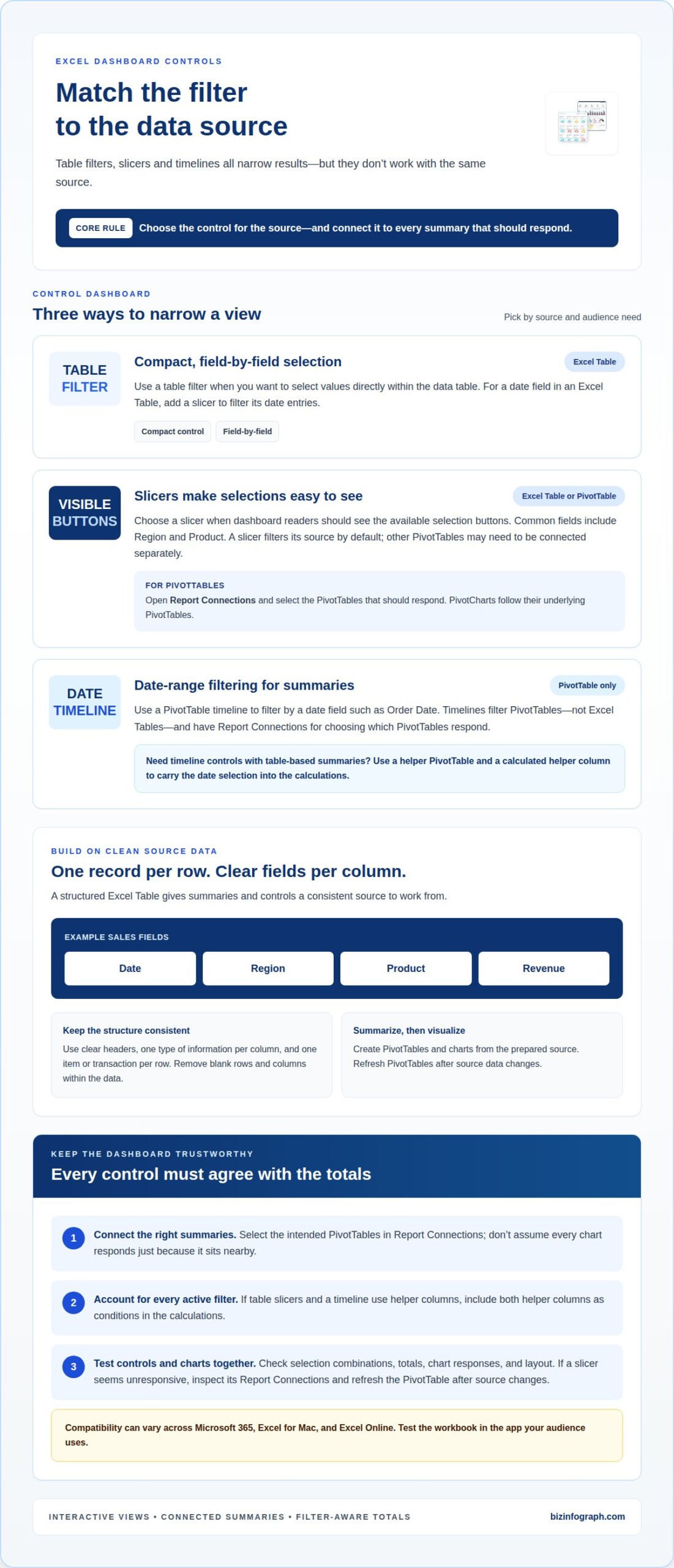
   PivotCharts reflect their underlying PivotTables, so connect the slicer to the relevant tables rather than relying on visual proximity. A timeline also has Report Connections for selecting PivotTables. Remember that timelines filter PivotTables, not Excel Tables. For date filtering on table-based summaries, a helper PivotTable can provide the timeline control.

3. Compare Slicers with Filters

   Use a table filter for compact, field-by-field selection within the data table. Choose a slicer when visible buttons make the current selection easier to understand on a dashboard. Both narrow results, but slicers provide a more prominent visual control for fields such as region or product.

   For time periods, use a PivotTable timeline rather than expecting an Excel Table to support one. PivotTables summarize records, but they can expand or contract as data and filters change, so leave room in the layout. Create a PivotChart from the summary, then choose a line chart to show trends or columns to compare values. Test the controls and chart responses together before sharing the dashboard.

What is an Excel dashboard used for?

An Excel dashboard brings key measures into one view for tracking sales, budgets, projects, or KPIs. Slicers and timelines make that view interactive, letting readers filter results instead of scanning every record.

1. Filter by the question your audience needs to answer. Add slicers for fields such as region or product, and use a PivotTable timeline to narrow results by Order Date. For example, a sales dashboard can show revenue for a selected region and date range, helping users compare the view they need.
2. Make each aggregation formula respect every active filter. If table slicers and a timeline use helper columns, include both helper columns as formula conditions. One helper can mark rows that match table selections; the other can return 1 for dates inside the visible timeline range and 0 otherwise. Omitting either condition can leave totals inconsistent with the filtered view.
3. For an Excel Table, add a slicer for a date field to filter its date entries. A PivotTable timeline does not filter the Excel Table itself. If the dashboard needs timeline controls alongside table-based summaries, use a helper PivotTable and a calculated helper column to carry the date selection into the calculations.
4. Format slicers by resizing them, choosing a Slicer Style, and arranging buttons in multiple columns. Compatibility can vary across Microsoft 365, Excel for Mac, and Excel Online, so test the workbook in the app your audience uses. If a slicer seems unresponsive, inspect its Report Connections, confirm it controls the intended PivotTable, and refresh the PivotTable after its source data changes. Test combinations of selections and check that charts, totals, and layout respond correctly before sharing.

Connecting and preparing spreadsheet data

Build a dashboard from a structured Excel Table: give each column a clear header and each row one record. For example, use Date, Region, Product, and Revenue fields, then summarize the source with PivotTables and charts.

1. Inspect the source before creating summaries. Keep one type of information in each column, such as dates in Date and sales amounts in Revenue. Remove blank rows and columns within the data, since gaps can interrupt the range Excel reads. Check that every record includes the fields your dashboard will use.
2. Make each row represent one item or transaction. In a sales dataset, a row might record a product sale in a region on a particular date. Don’t combine several products in one row or place totals among the records. A consistent row structure helps PivotTables group and summarize data accurately.
3. Convert the cleaned range into an Excel Table. Select a cell in the data and press Ctrl+T, then confirm the range and that the table has headers. The table can expand when you add rows, giving later summaries a source that grows with the dataset. Clear headers also become useful field names in PivotTables and slicers.
4. Clean or reshape imported data with Power Query before building the dashboard. Use it to organize fields into a consistent table, then confirm that Date, Region, Product, and Revenue remain separate columns. These fields can support different views, such as revenue by product or region, without rebuilding the source for each chart.
5. Create a PivotTable from the prepared table and assign fields to answer your question. For a monthly product view, place Date in Rows, Product in Columns, and Revenue in Values, then group dates by month and year. Add a chart and slicers once the summary is sound. When new records arrive, refresh the PivotTable so its results reflect the updated source.

How to create an Excel dashboard with slicers step by step

1. Start with the prepared source table and decide which questions the dashboard should answer. For a sales view, choose measures such as revenue and dimensions such as date, product, and region. Sketch the key visuals first, so each PivotTable and chart has a clear purpose instead of repeating the same comparison.
2. Create a PivotTable from the source and assign fields to suit one visual. For example, place Date in Rows, Product in Columns, and Revenue in Values. Group dates by month and year to reveal movement over time. Build separate summaries when a chart needs a different arrangement, such as comparing revenue across regions.
3. Insert a chart for each PivotTable summary and choose a format that suits the comparison. A line chart shows trends across months, while a clustered column chart compares products or regions. Give each chart a clear title and consistent number formatting, then position the visuals so viewers can scan results without confusing one measure for another.
4. Add slicers for fields people will commonly explore, such as Product and Region. Open each slicer’s Report Connections and connect it to every relevant PivotTable. If the dashboard needs date navigation, add a timeline to a PivotTable and connect it through Report Connections. Test a product selection and a date range to confirm the intended charts update together.
5. Arrange the charts, slicers, and summary figures on one dashboard sheet. Leave room for PivotTables to expand or contract as selections change, and keep controls beside the visuals they affect. Refresh PivotTables after source data changes, then test several filter combinations before sharing. For a ready-made starting point, explore Excel dashboard templates and adapt the layout to your reporting needs.

Biz Infographs: PowerPoint Infographic Templates

Biz Infographs offers Excel Dashboard Templates for readers who want a polished starting point for presenting data. They can help you move from a working dashboard to a clearer visual layout, while Excel Charts support focused data comparisons. If your reporting needs extend beyond Excel, Power BI Templates and Automation Templates offer related options for visualizing data and streamlining spreadsheet work.

Choose a template when you want to spend less time arranging dashboard elements and more time shaping insights for your audience. Adapt the layout to your measures, charts, and filter controls, then refine it for your reporting needs. For presentation-focused visuals, explore PowerPoint Infographic Templates to communicate key findings beyond the spreadsheet.

Visit bizinfograph.com to explore the templates and choose a starting point for your next dashboard.

Put your dashboard to work

A well-designed Excel dashboard with slicers should support a real decision, not simply display polished charts. Choose one recurring question your team needs to answer, then use the dashboard during that review. Notice which views people rely on and where they still need clarification. Those observations can guide your next refinement, from adjusting a visual’s emphasis to making a key comparison easier to spot.

Keep the dashboard useful as reporting needs evolve. Revisit its measures and layout when priorities change, and make the next improvement based on how people use the information. A focused dashboard can turn routine reporting into a clearer conversation about what to do next.

Ready to develop your dashboard further? Contact Biz Infographs for dashboard help and take the next step toward presenting your data with confidence.

Frequently Asked Questions

How do I add slicers to PivotTables and PivotCharts in Excel?

Select a cell inside the PivotTable, choose the slicer command, and select the field viewers should filter, such as Region. The slicer controls that PivotTable, and its associated PivotChart reflects the filtered results. To show several regions together, hold Ctrl while selecting slicer buttons. Use the clear-filter control to restore the full view.

How do I connect one slicer to multiple PivotTables in Excel?

Select the slicer, open Report Connections, and tick the PivotTables it should control. Then click a slicer button and compare the affected summaries to confirm each responds as intended. A slicer initially controls the PivotTable it was created for, so this connection step is essential when your dashboard presents separate summaries, such as sales by product and sales by region.

How do I use timelines and date slicers in Excel dashboards?

Add a timeline to a PivotTable that contains a date field, then select the date range to filter its results. Use Report Connections to apply the timeline to other relevant PivotTables. Excel Tables don’t support timelines directly; for a table-based dashboard, a helper PivotTable and calculated helper column can pass the date selection into dashboard calculations.

What are best practices for designing an interactive Excel dashboard with slicers?

Give each chart and slicer a clear role, and leave space between charts so controls don’t crowd the data. Keep PivotTables far enough apart to expand or contract without overlapping. Test combinations of slicer and timeline selections before sharing, checking that totals and charts agree. For example, select one product and a date range, then confirm every relevant visual updates.