Introduction to Drop Down List in Excel
What is a Drop Down List in Excel?
A drop-down list in Excel is a powerful feature that allows users to select a value from a predefined list. This tool enhances the user experience in spreadsheets by standardizing entries and minimizing input errors. The drop-down list in Excel worksheet is created using the data validation feature, which restricts the cell to values only within a specified source list. Whether you’re creating a drop-down for a form, a checklist, or data categorization, this function is essential for improving data integrity. You can create a dropdown using either a simple list of items separated by a comma or a dynamic list linked to a named range. Excel will display a drop-down box that users can interact with by clicking on a cell.
Benefits of Using Drop-Down Lists in Spreadsheets
Using drop-down lists in Excel can dramatically improve your data management experience. These dropdowns help standardize entries across your spreadsheet, reduce user errors, and speed up data entry. When you insert a drop-down list, users can only choose from the allowed items, preventing incorrect or inconsistent values. This is especially helpful when working with long forms or shared documents. With features like the invalid data is entered box in Excel data validation, users are prompted if they try to enter incorrect data. A drop-down list allows quick selection, making it ideal for both short and longer lists, and is widely used in Microsoft Excel across industries.
Common Use Cases for DropDown List in excel
Drop-down lists are widely used in a variety of real-world scenarios. In HR, dropdowns help standardize department names or job titles. In inventory management, drop-down boxes list predefined product categories. In finance, they might define payment terms or invoice statuses. A simple drop-down list can be created from comma separated values for short lists, while dynamic drop-down lists are used when the number of values changes frequently. Using drop-down lists ensures consistent data collection and makes it easier to analyze results later. You can also use a dependent drop-down list when one selection depends on another, such as selecting a region and then a city.
How to Create a Simple Drop-Down List in Excel
Select the Cell Where You Want the Drop-Down
To begin creating a drop-down list in Excel, first click on a cell or multiple cells where you want the dropdown to appear. This is where users will select an item from a list. You can use drop-downs in a single column or row without affecting other parts of your spreadsheet. Once you’ve made your selection, you’ll proceed to insert a drop-down list using the data validation dialog box tool. It’s essential to choose your location thoughtfully to ensure it aligns with your spreadsheet’s purpose and layout. The drop-down box will only appear in the selected cells and can be customized using Excel’s data validation settings.
Using Data Validation to Create Your Drop-Down
After selecting the target cell(s), go to the Data tab and choose “Data Validation.” This tool is your gateway to using drop-down lists in Excel. In the data validation settings window, under the Allow drop-down, select “List.” In the Source box, type your list of items separated by a comma (e.g., Low, Medium, High). Excel will use this list to populate the drop-down. This method is ideal for short, predefined lists and offers a quick way to ensure that data entered follows a consistent format. Excel will display a drop-down arrow in the cell, allowing users to select a value and improving data accuracy.
Entering Comma Separated Values for Your Select List
When creating a drop-down list in Excel for short lists, you can enter your source list directly into the data validation settings using comma separated values. For example, typing “Red, Blue, Green” into the source box will populate your drop-down with these options. This is a fast and effective way to create a drop-down for a fixed number of values. This method works well when you do not expect to add or remove items frequently. Excel will automatically create a drop-down list based on this text input, allowing users to select from the available items when entering data.
Creating Drop-Down Lists from a Named Range
How to Define a Named Range in Excel
A named range in Microsoft Excel is a user-defined label for a range of cells that can be used in formulas and data validation. To create one, enter your list of items into a column, then highlight the cells and go to Formulas > Define Name. Assign a unique and meaningful name, such as “ProductList”. This named range becomes the source for your drop-down list. Using a named range is especially helpful when creating a drop-down in Excel that you want to reuse or reference across multiple cells or sheets. It also supports creating a dynamic list that updates automatically when new items are added.
Select Data Validation and Link to the Named Range
Once you’ve created your named range, go back to your spreadsheet, click on the cell where you want the drop-down, and select Data Validation. Choose “List” under the Allow section. In the Source box, enter the named range with an equal sign (e.g., =ProductList). This links your drop-down directly to the list of items you created earlier. Now, when you or someone else clicks on that cell, Excel will display the options from the named range. If you add new items to the source list and the range is dynamic, those items will automatically be added to the drop-down list.
Managing and Editing Your Named List in Excel
Managing a named list in Excel is simple and efficient. If you need to add or remove items from a drop-down list, go to the named range and update the contents directly. For dynamic lists, it’s recommended to convert your source list into a table by selecting it and choosing Insert > Table. Excel will automatically extend the range when you add new items to the table. If the list is not dynamic, you’ll need to manually redefine the named range when adding or removing entries. This flexibility makes named ranges ideal for creating a drop-down that evolves over time.
How to Create a Dependent Drop-Down List in Excel
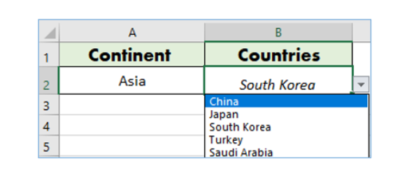
What is a Dependent Drop-Down List?
A dependent drop-down list in Excel is a drop-down whose items change based on the selection made in another drop-down. This is useful when you have related categories, such as “Country” and “City” or “Category” and “Subcategory.” For instance, when you select “Fruits” in the first drop-down list, the second drop-down will only show fruits like “Apple” or “Banana.” This technique is also known as cascading or conditional dropdowns. Dependent drop-downs are built using named ranges and Excel functions like INDIRECT to reference the source list dynamically, making data entry more context-aware and efficient.
Setting Up the Primary and Dependent Lists
To create a dependent drop-down list, first prepare your primary list (e.g., Product Types) and then create separate lists for each category in the second drop-down (e.g., Laptops, Desktops under Electronics). Name each secondary list exactly the same as its corresponding primary item. Next, create your first drop-down list using standard data validation. For the dependent drop-down, use the formula =INDIRECT(A2) in the data validation source box, where A2 is the cell containing the first drop-down. Excel will use the selection in the first drop-down to determine the list for the second drop-down, allowing you to select a value specific to your previous choice.
Using Named Ranges and INDIRECT Function
The INDIRECT function is key to building a dependent drop-down in Excel. This function takes the text value of a cell (like the first drop-down’s selection) and converts it into a reference for the second list. For example, if cell A2 contains “Fruits,” and you have a named range called “Fruits” listing Apples, Oranges, and Bananas, using =INDIRECT(A2) in the second drop-down’s data validation will populate it with those fruit options. It’s important that the names of your dependent lists match exactly with the entries in the first list. This method is one of the most flexible ways to create your drop-down relationships in Excel.
Creating a Dynamic Drop-Down List
Why Use Dynamic Lists in Excel?
A dynamic drop-down list in Excel automatically updates when you add new items to the source list. This is essential for data entry scenarios where the list of available options can change over time. Dynamic lists improve efficiency by removing the need to manually update the drop-down each time you modify the source. This is especially useful in shared spreadsheets where data is frequently updated. By using a table or a formula-based named range, Excel will display new items from the list automatically. This results in better workflow automation and an overall enhanced data validation experience.
How to Create a Dynamic Range Using Excel Formulas
To create a dynamic list using a formula, first place your items in a single column. Then go to Formulas > Name Manager and create a new named range. Use a formula like =OFFSET(Sheet1!$A$2,0,0,COUNTA(Sheet1!$A:$A)-1) to dynamically define the list. This formula calculates the number of non-blank cells and adjusts the list accordingly. Alternatively, convert your list into a Table using Insert > Table. Tables expand automatically when you add new rows, making them ideal for dynamic drop-down lists. Excel data validation can reference this named range or table to populate the drop-down box with the most current items.
Linking the Dynamic Range with Data Validation
After you’ve created your dynamic named range or Excel Table, it’s time to link it with data validation. Click on a cell where you want the drop-down, then go to Data > Data Validation. In the settings, select “List” and enter the named range in the Source field, using the equal sign (e.g., =MyDynamicList). Now, when you add new items to the source list, they will appear automatically in the drop-down. This approach ensures your dropdown list remains current without manual updates. It’s especially beneficial for longer lists or databases where list items from a drop-down list may change frequently.
For ready-to-use Dashboard Templates: